By Chris Rollins, Ph.D., Michigan State University; Ross S. Stein, Ph.D., Temblor; Guoqing Lin, Ph.D., Professor of Geophysics, University of Miami; and Deborah Kilb, Ph.D., Project Scientist, Scripps Institution of Oceanography, University of California San Diego
A new image of the ground deformation, a rich and enigmatic foreshock sequence, aftershock trends we can explain, and others that are more elusive. This is also the time see how Temblor app’s hazard forecast for Ridgecrest fared.
Citation: Chris Rollins, Ross S. Stein, Guoqing Lin, and Deborah Kilb (2019), The Ridgecrest earthquakes: Torn ground, nested foreshocks, Garlock shocks, and Temblor’s forecast, Temblor, http://doi.org/10.32858/temblor.039
For a note on what to do during an earthquake (re: Jimmy Kimmel’s segment), see the end of this article.
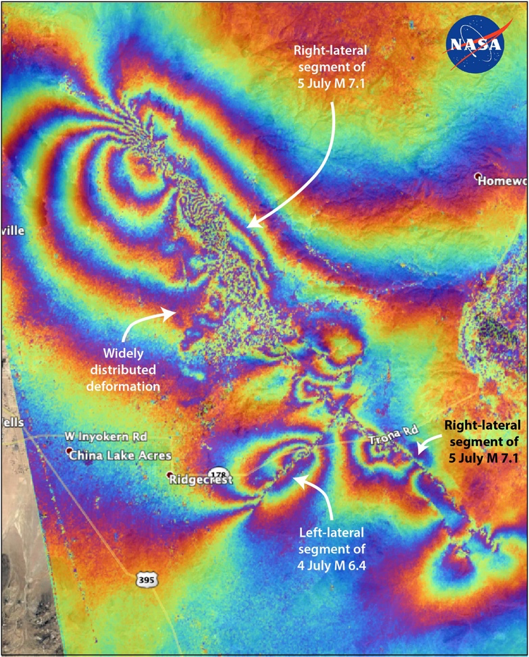
Ground Deformation from Space
The Advanced Rapid Imaging and Analysis (ARIA) team at NASA JPL and Caltech just released this Interferometric Synthetic Aperture Radar (InSAR) image that shows how the fault slip in the 4 July M 6.4 and 5 July M 7.1 earthquakes warped the earth’s surface. We have annotated the map to highlight its remarkable features: knife-edge faulting in the south, and what looks like a distributed band of shear in the north. That broad pattern of deformation may explain why geologists had missed the fault in the first place: it may masquerade as several small, discontinuous tears at the surface. By using this image and others like it that will come in as more radar satellites pass over the Ridgecrest area, we can study how the slip in these earthquakes was distributed at depth, why the fault may have slipped that way, and what that might mean for how earthquakes occur in general.
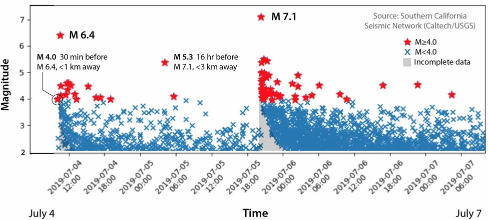
Foreshocks of foreshocks
When we look how the earthquake sequence unfolded in time, we see what we might call ‘nested foreshocks.’ First, a M 4.0 struck 30 min before the M 6.4 mainshock in virtually the same location. Rare, but not unprecedented. About 18 hours into the M 6.4 aftershock sequence, the largest aftershock, a M 5.3 event struck. Then, about 16 hours later, the M 7.1 ruptured less than 3 km from the site of the M 5.3. That’s also rare. But while fascinating, we don’t see much that marks those little shocks for future greatness.
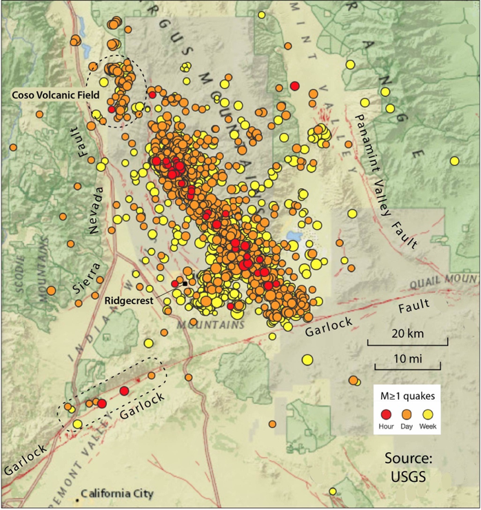
Aftershocks in the Coso Volcanic Field and on the Garlock Fault
The Coso Volcanic Field, an area northwest of the earthquake with a history of seismic swarms, has lit up in earthquakes since the 7.1 quake. Over the past 48 hours, aftershocks have also begun to show up along parts of the Garlock Fault to the southwest. Can we explain these observations?
When an earthquake ruptures a fault, it warps the surrounding earth (as captured by the satellite image above) and therefore changes the state of stress in the earth around it, including along nearby faults. These stress changes can push some faults closer to failure and pull others further from it, depending on where they are with respect to the earthquake. In the plot below, we used the USGS slip model for the M 7.1 shock to calculate what it might have done to the major mapped faults in the region and others oriented like them. All else being equal, we would expect aftershocks to be more numerous around faults brought closer to failure by the stress changes in the M 7.1 earthquake (the red zones below), and less prevalent along faults inhibited from failure (the blue ‘stress shadows’).
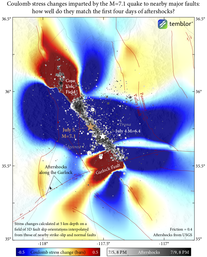
We see that the the 7.1 quake likely brought faults in the Coso Volcanic Field closer to failure, consistent with the abundant aftershocks there. But although the quake also strongly increased the Coulomb stress on a 30-km (20-mile) stretch of the Garlock, most of the aftershocks along the Garlock have in fact appeared in a blue zone to the southwest. Satellite radar imagery spanning several years before these quakes suggests the Garlock may be slowly creeping in the blue zone [Tong et al., 2013], which if real could play into seismicity there, but that signal is within the noise level of the dataset. Satellite radar imagery and other geodetic (surface deformation) data and field observations will help piece together what has been going on, not only near the Garlock but everywhere in and around the Ridgecrest sequence.
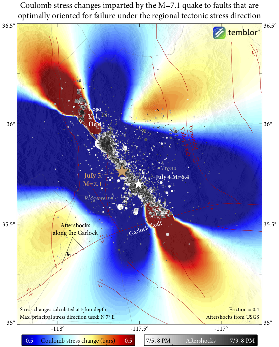
It is also possible that some of those aftershocks to the southwest didn’t actually occur on the Garlock, but instead on smaller nearby faults that are more optimally oriented for failure under the current tectonic stressing that drives the Eastern California Shear Zone. (The Garlock, for its part, has been rotated severely out of alignment with the regional stress direction, so exactly how much and how often it still slips is a topic of ongoing research.) The above plot shows that faults with this more optimal orientation would have in fact been slightly promoted for failure by the Ridgecrest quake down around where those aftershocks are occurring. We see that faults oriented like this in the Coso region would also have been in the red.
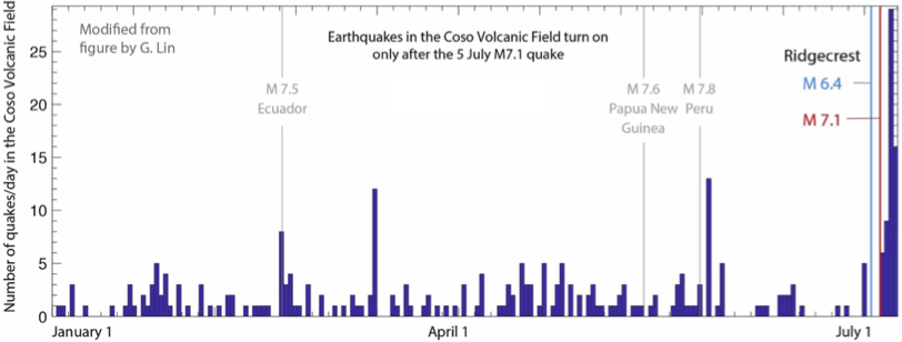
A closer look at Coso shows that, intriguingly, it was quiet after the M 6.4 4th of July earthquake, but began to light up in earthquakes as soon as the M 7.1 hit on July 5. That might be because the 7.1 was a much larger earthquake and induced larger Coulomb stress changes there; it might alternatively (or also) be because the throughgoing seismic waves from the 7.1 shook Coso harder. We note that a M 7.5 earthquake in Ecuador earlier this year may have also been correlated with a temporary uptick in seismicity in Coso, but two other large remote earthquakes don’t look like they were. This effect, called remote triggering, has been observed in various parts of the world following several large earthquakes in the past 25 years, but studies differ on whether it is characteristic of the Coso region [Castro et al., 2017; Zhang et al., 2017]. Nevertheless, with more in-depth research, we can use the Ridgecrest sequence and Coso aftershocks as a natural experiment that helps shed light on what controls earthquake behavior there – and therefore what may control it in general.
How useful was Temblor in offering guidance to Ridgecrest residents?
Temblor gives three condensed forecasts in one screen. Here it is, slightly annotated:
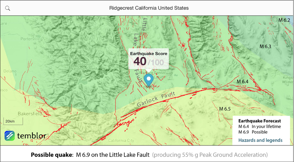
– Earthquake Score is 40, which is based on the most current ‘probabilistic’ USGS model. A score of 100 means probable damage of 20% of the replacement cost of a home in 30 years. The score factors in all quakes large and small, near and far, and the amplification of shaking in basins. For comparison, the score is 65 in downtown Los Angeles, and 95 in San Bernardino.
– Lifetime quake is M 6.4. This is the earthquake magnitude that has a 1% chance per year of occurring within 60 mi (100 km); that’s a 60% chance of occurring if you live to 90. It was certainly exceeded, and this tells us that a M 7.1 here is rare. The lifetime quake is M 6.7 for L.A., and M 6.8 for San Bernardino.
– Possible quake is M 6.9. Temblor finds the USGS ‘scenario’ earthquake that produces the strongest shaking at your location and reports its magnitude, fault, and the shaking. Temblor then estimates the cost of repairing the damage to your home in this quake, based on your home’s characteristics. For L.A., it is M 7.0, and for San Bernardino, it is M 7.7. Although the shaking estimate is for a nearby fault with a lower magnitude, it turns out to be spot on: The forecast peak shaking was 55% g (55% of the force of gravity) and the observed was 57%.
Why do we give you two quake magnitudes? (in this case, M 6.4 and M 6.9). The first is the quake size you will more likely than not experience in your lifetime, the second is the largest that the USGS considers possible at your location. On July 5, both were exceeded, but the forecasted shaking nevertheless turned out to be prescient.
In short, while earthquakes will continue to surprise us, their shaking doesn’t have to. Take this opportunity and understand your risk.
A note on what to do when the earthquake strikes (and when you get a ShakeAlert alert)
Jimmy Kimmel got it almost right – the “triangle of life” idea is indeed wrong and doorways aren’t all that great – but you should still definitely get under a table or desk in an earthquake, if one’s close by. That’s never changed, and it’s a key part of “cover” in drop, cover, and hold on. Check out Dr. Lucy Jones’ interview on Conan – she shows a picture from the 1985 Mexico City earthquake of a concrete ceiling that collapsed but was held up by a few school desks. That’s why getting under a table or desk is such a good idea.
References
Castro, R. R., Clayton, R., Hauksson, E., & Stock, J. (2017). Observations of remotely triggered seismicity in Salton Sea and Coso geothermal regions, Southern California, USA, after big (MW> 7.8) teleseismic earthquakes. Geofísica internacional, 56(3), 269-286.
Tong, X., Sandwell, D. T., & Smith‐Konter, B. (2013). High‐resolution interseismic velocity data along the San Andreas fault from GPS and InSAR. Journal of Geophysical Research: Solid Earth, 118(1), 369-389
Zhang, Q., Lin, G., Zhan, Z., Chen, X., Qin, Y., and Wdowinski, S. (2017). Absence of remote earthquake triggering within the Coso and Salton Sea geothermal production fields. Geophys. Res. Lett., doi:10.1002/2016GL071964.
Ph.D., California Institute of Technology, 2017