Between Los Angeles and San Francisco, the San Andreas Fault releases stress by gradual movement. Scientists calculate fault slip from offset topography and discuss seismic hazard.
By Chelsea Scott, Ph.D., Assistant Research Scientist, Arizona State University (@ChelseaPScott)
Citation: Scott, C., 2021, The Central San Andreas creeps along without a major earthquake, Temblor, http://doi.org/10.32858/temblor.152
The San Andreas Fault in California is well known for generating large and damaging earthquakes — including the 1906 magnitude 7.8 San Francisco earthquake. Perhaps less well known, is the fact that some portions of the San Andreas Fault rarely, if ever, rupture in large earthquakes. Between Los Angeles and San Francisco, for example, a portion of the San Andreas Fault continuously slips, or “creeps” at a rate of approximately three-quarters of an inch (20 millimeters) per year. A creeping fault can generate small earthquakes, but shaking is generally imperceptible or felt only near the fault. Occasionally, a creeping fault can suddenly slip in a large earthquake.
In a new study published in Geophysical Research Letters, my colleagues and I show where and how much this fault is creeping. We use airborne instruments to measure changes in topography that are too small and occur too slowly for our eyes to see. These new observations reveal the active trace of the creeping San Andreas Fault and show the extent to which the active motion hugs a narrow fault trace. These constraints are critical for scientists to understand the processes that control fault creep in the crust and to determine seismic hazard.
Creeping faults are a hazard
Because creeping faults slip gradually and nearly continuously, they do not build up as much stress as locked faults, which slip infrequently and release a majority of stress in large earthquakes. However, creeping faults do build some stress, which is often not fully released, meaning that these faults can host large earthquakes and pose a hazard. Measuring fault activity or the creep rate is essential for knowing how much stress is built-up along these faults and the likelihood of a moderate to large earthquake in the future.

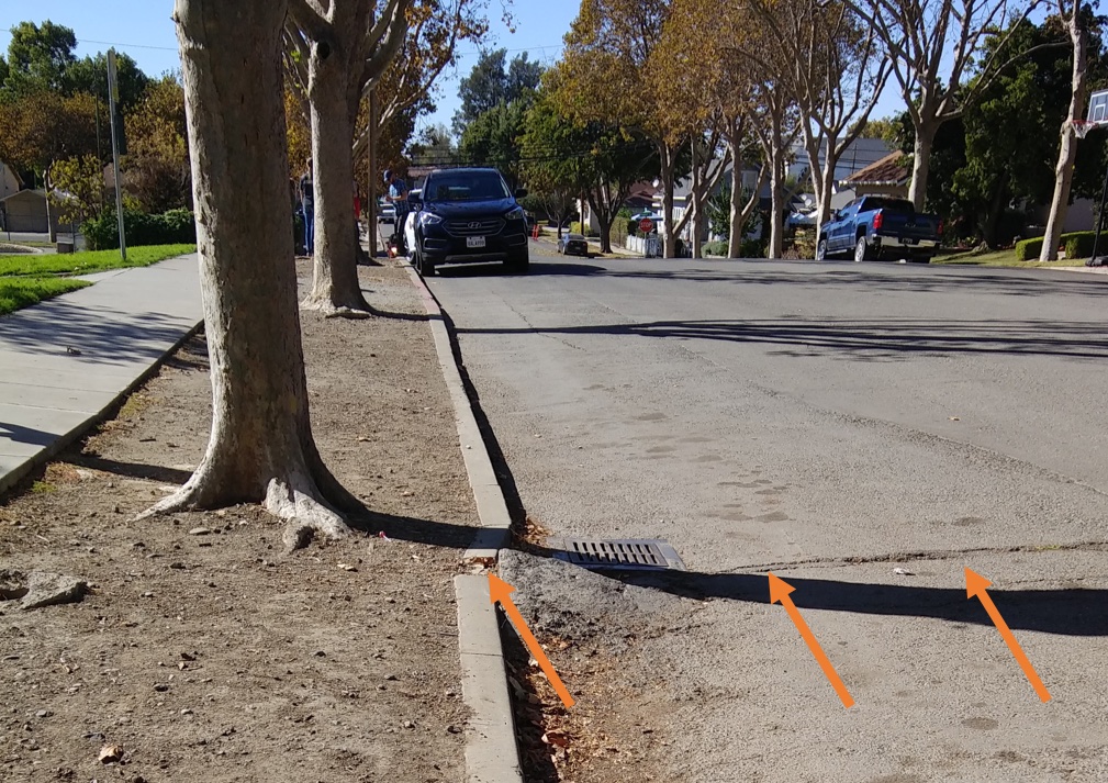
Measuring fault motion from a shifting landscape
Measuring a fault slip rate is challenging. Offset curbs like the one pictured above in Hollister, California, give scientists a way to directly observe how much slip has occurred in a given location, but these types of structures do not cross the fault at the spacing required to accurately measure large-scale fault motion. There are a variety of approaches for measuring fault slip rate, but most do not capture a spatially dense slip rate that is critical to assessing the fault’s overall activity.
Light detection and ranging, known as lidar, is a technique used to create a three-dimensional representation of a target based on a laser signal. Although well-known for its use in self-driving cars, geologists use this technique to measure elevation across a landscape. When the elevation surrounding a fault is measured at two different times — often months to years apart — comparing the two topography datasets reveals how the has fault moved (Nissen et al., 2012; Oskin et al., 2012).
My colleagues and I were the first to measure the fault creep rate along the entire creeping portion of the Central San Andreas Fault from airborne lidar datasets. This work resulted in the most spatially dense slip rate measurements along the fault available. We measured the right-lateral creep rate every 1300 feet (400 meters) along the fault from airborne lidar topography datasets acquired just over a decade apart. Applying this method to a creeping fault was challenging because the decade of fault creep produced a relatively low amount of slip relative to the noise in the data. To decrease the noise and better resolve the creep, we removed vegetation from the lidar data because changes in vegetation contribute significantly to the noise.

Not all tectonic motion occurs along a discrete fault
The motion between two sides of a fault can either be localized to a narrow surface or distributed over a broader region in the Earth’s shallow crust. Research on earthquakes has shown that older faults that have accommodated more slip tend to localize motion to a narrow fault. The San Andreas Fault is very old and should localize roughly 90% of the motion to the fault trace (Dolan & Haravitch, 2014). However, we show that only 50-80% of the motion along the creeping San Andreas Fault occurs on a narrow fault trace. We propose that this unexpected behavior reflects the much slower slip rate during creep events relative to earthquakes.

Which fault is active?
Our results show a picture of motion within a mile surrounding the fault trace that allows scientists to clearly see which faults in the Earth’s shallow crust accommodate motion. In the right figure above, we trace out the active San Andreas fault in black based on the fault’s motion over the past decade. This active fault trace is approximately half of a mile away from where the US Geological Survey mapped the fault based on the shape of hills and valleys that indicate an older fault location. The different fault locations show that the active trace of the San Andreas fault has shifted over time. Critically, our result reveals the location of the fault active over the past decade, which is an important input into seismic hazard assessment.
Seismic risk
The stress buildup along a fault depends on the difference between the long-term tectonic plate boundary rate and the creep rate. One of the major challenges in measuring the seismic risk is knowing how fault slip rates change from the surface where they can be measured to the deeper portions of the fault where slip rates are much more challenging to measure. To infer the slip rate at depth, scientists look at surface motion over a larger area, which indicates deeper fault slip. These displacements measure fault slip at a scale between very near-field and far-field instruments. In the future, we plan to use surface motion measurements over a range of areas to infer fault slip over the entire subsurface extent of the fault. This analysis will indicate the stress buildup and the likelihood of a future earthquake along the fault.
Further reading
Dolan, J. F., & Haravitch, B. D. (2014). How well do surface slip measurements track slip at depth in large strike-slip earthquakes? The importance of fault structural maturity in controlling on-fault slip versus off-fault surface deformation. Earth and Planetary Science Letters, 388, 38–47. https://doi.org/10.1016/j.epsl.2013.11.043
EarthScope (2008). EarthScope Northern California LiDAR Project. NSF OpenTopography Facility. https://doi.org/10.5069/G9057CV2
Nissen, E., Krishnan, A. K., Arrowsmith, J. R., & Saripalli, S. (2012). Three-dimensional surface displacements and rotations from differencing pre- and post-earthquake LiDAR point clouds. Geophysical Research Letters, 39(16). https://doi.org/10.1029/2012GL052460
Oskin, M. E., Arrowsmith, J. R., Corona, A. H., Elliott, A. J., Fletcher, J. M., Fielding, E. J., et al. (2012). Near-Field Deformation from the El Mayor-Cucapah Earthquake Revealed by Differential LIDAR. Science, 335(6069), 702–705. https://doi.org/10.1126/science.1213778
Scott, C. P., DeLong, S. B., & Arrowsmith, J. R. (2020). Distribution of Aseismic Deformation Along the Central San Andreas and Calaveras Faults from Differencing Repeat Airborne Lidar. Geophysical Research Letters. https://doi.org/10.1029/2020GL090628
- Venezuela’s doublet leaned toward Caracas - June 30, 2026
- Is Southern California’s Cajon Pass an ‘earthquake gate’ ready to open? - June 29, 2026
- Philippines magnitude 7.8 shock may have loaded the central Cotabato subduction zone - June 11, 2026