Forecasting aftershocks: Back to square one after a Deep Learning anticlimax

By Arnaud Mignan, Ph.D. (@ArnaudMignan), ETH Zurich, Switzerland; Risks-X, SUSTech, Shenzhen, China
 
What went wrong in a much-heralded analysis designed to forecast aftershocks? The use of Artificial Intelligence made a simple problem overly complex.
 
Citation: Mignan, Arnaud (2019), Forecasting aftershocks: Back to square one after a Deep Learning anticlimax, Temblor, http://doi.org/10.32858/temblor.053
 

Aftershock patterns can be characterized in time, space, magnitude, and their relation to mainshock magnitude by some well accepted empirical laws. It is these laws, constrained by abundant data, that allow us to forecast aftershocks with some confidence (see e.g., Reasenberg & Jones, 1994; Gerstenberger et al., 2005).

A 2018 study published in Nature by Phoebe DeVries and her colleagues at Harvard and Google claimed that Deep Learning was able to predict the locations of aftershocks with accuracies far greater than Coulomb stress transfer could achieve

DeVries et al. (2018) was celebrated in the media (e.g., New York Times, 2018; USA Today, 2018; Futurism, 2018; The Verge, 2018) and Nature itself was unusually definitive in its coverage of the article: “Artificial intelligence nails predictions of earthquake aftershocks” (Witze, 2018). But does it, really? The recent ‘Matters Arising’ Comment by Marco Broccardo and myself (Mignan & Broccardo, 2019b), which was replied to by senior author Brendan Meade (Meade, 2019), argues that it doesn’t, and that we are back to square one in our capacity to forecast the distribution of aftershocks around a mainshock rupture.

Here I present the two papers (the original Nature paper and its comment) and put them into the wider context of Statistical Seismology on one hand, and of Deep Learning on the other. To fully appreciate this article, I recommend readers to first watch the next video, which summarizes the original Deep Learning study and sets the problem in simple terms. It also provides a preliminary “shallow learning” alternative, which led to the conference paper Mignan & Broccardo (2019a) in mid-2019 (part of the Lecture Notes in Computer Science book series).

 

Video by Arnaud Mignan, dated 20 January 2019, describing the DeVries et al. study, the problematics on using deep learning for the prediction of aftershocks in space, and some alternatives based on “shallow learning” (read Mignan & Broccardo (2019a) for more details).
 
How seismologists think about aftershocks

Simply put, aftershocks are most likely near the mainshock rupture, and the probability to see aftershocks decays with the distance from the mainshock or the fault rupture surface. This pattern is quantified by one of a handful of empirical laws available in Statistical Seismology: Omori proposed his famous temporal power-law in 1894, extended in 1961 by Utsu. It is again Utsu, in 1970, who first proposed the productivity exponential law linking number of aftershocks to the mainshock magnitude. He did it by combining two other important laws of Statistical Seismology, the Gutenberg-Richter law of 1944 and Båth’s law of 1965 (for an explicit demonstration, see Mignan, 2018).

 

 

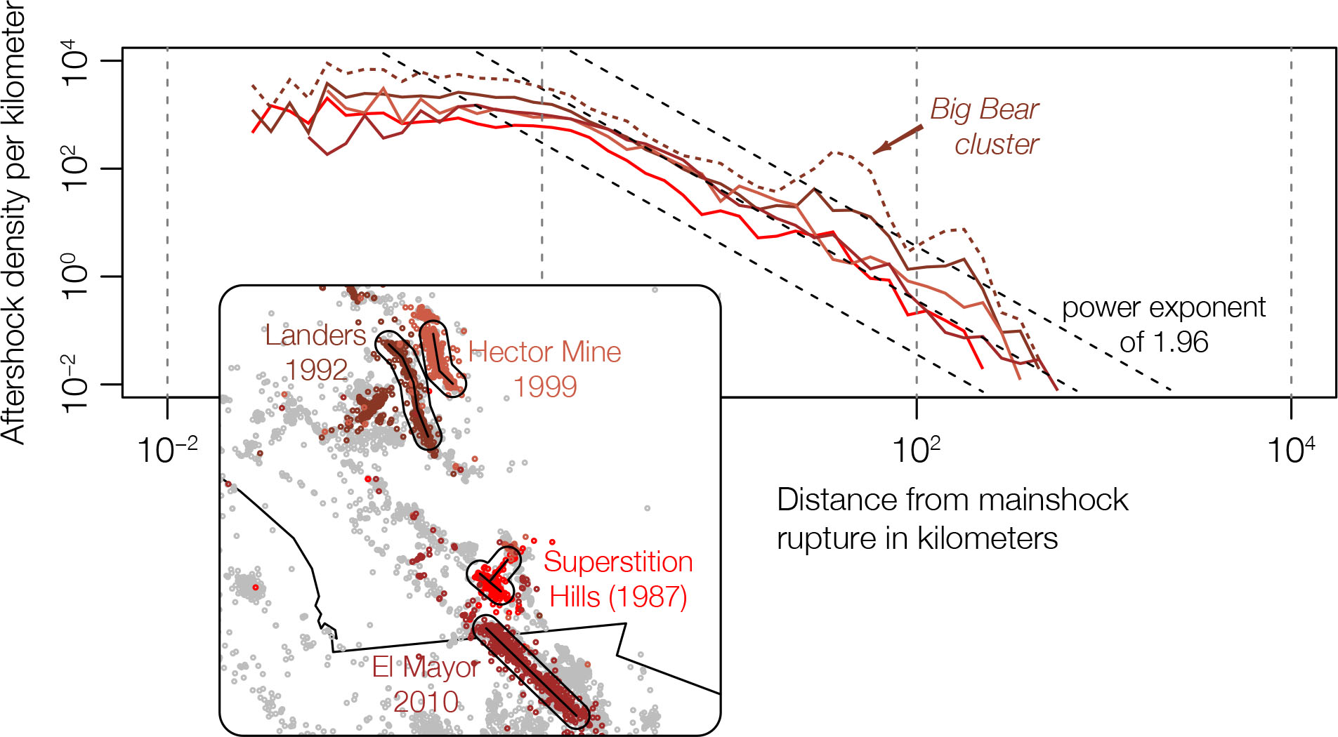
Although we cannot trace it back to one specific publication, a ‘power-law’ decay of aftershock density with distance from the mainshock is commonly accepted in the Statistical Seismology community. Knopoff was perhaps its main investigator (Kagan & Knopoff; 1980; Yamashita & Knopoff, 1987) but both power-law and Gaussian kernels were still in use in the 1990s (e.g., Ogata, 1998). Today, the power-law behavior has been verified by a number of studies (e.g., Richards-Dinger, 2010; Hainzl et al., 2010 and references therein). This is illustrated in the next figure for the largest strike-slip mainshocks in southern California (Mignan, 2018). When we return to the study of DeVries et al., it will be important to ask ourselves whether Deep Learning can really extract any pattern that is not already simply encoded by the distance to the mainshock rupture.

 

 

Harnessing Deep Learning by turning aftershock maps into a computer-vision problem

Deep Learning is best summarized by Yann LeCun, Yoshua Bengio and Geoffrey Hinton, the 2018 recipients of the Turing Award, the equivalent of the Nobel Prize for Computer Science: “Deep learning allows computational models that are composed of multiple processing layers to learn representations of data with multiple levels of abstraction. These methods have dramatically improved the state-of-the-art in speech recognition, visual object recognition, object detection and many other domains” (LeCun et al., 2015).

DeVries et al. used a ‘fully-connected’ (or dense) Deep Neural Network (DNN) made of 6 hidden layers, each composed of 50 ‘neurons.’ With additionally 12 input features (based on the earthquake-induced stress field – we will come back to this), their DNN had 13,451 free parameters, meaning a model of immense flexibility. One familiar with Machine Learning may find two issues with this specific ‘architecture,’ or experimental design. To understand the problem, let us take a detour by a textbook computer-vision example, and build a dense DNN to predict the class of the images in the MNIST database. MNIST (Modified National Institute of Standards and Technology) is a large database of handwritten digits that is commonly used for training various computer vision models. It is composed of 60,000 training images and 10,000 testing images (LeCun et al., 1998).

 

 

Let us build a DNN composed of an input layer, two hidden layers (hence deep), and one output layer. The model is presented as a Keras code snippet since this front-end to Google’s TensorFlow is as simple as a Lego construction (both DeVries et al. and Mignan & Broccardo used Keras). The next DNN architecture comes from https://keras.io/examples/mnist_mlp/

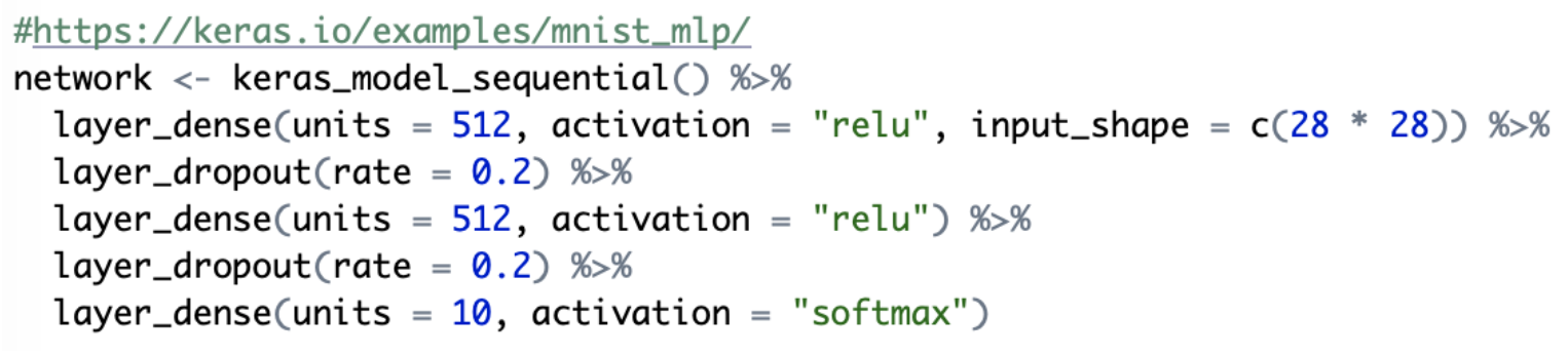
This model is composed of two hidden layers (layer_dense) with 512 neurons, or units, each. The input layer is implicit (input_shape) and is made of 28 times 28 neurons, i.e. 784 input parameters representing the pixels of each image. This is called image flattening, and we will come back to this very soon. The output layer (the last layer_dense) is composed of 10 neurons, representing the different digit labels, from 0 to 9, to be classified. When trained on some labelled data, the neural network modifies the weights of each neuron to fit, mimic, the handwritten digits so that when a similar pattern is later on observed, the network will predict (with some degree of accuracy) the correct label, i.e., the correct digit. This DNN leads to an accuracy of ~98.4% on the independent test set. The selection of the number of units per layer is quite flexible. From https://keras.rstudio.com/, we have:

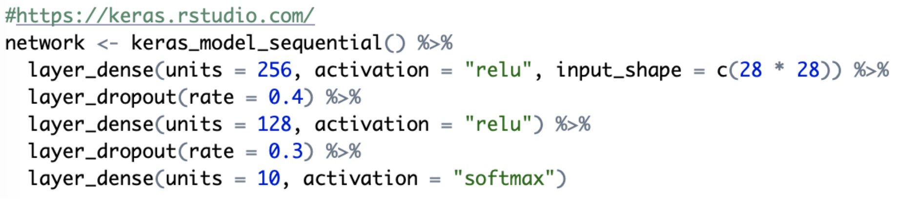
and get an accuracy of ~98.2%, so almost the same result, despite the change in the architecture.

The simplest of handwritten characters, such as “1” or “7”, may look similar to aftershock patterns taken in map view (look at the contour patterns in the southern California map of aftershock sequences). Taking some examples from the DeVries et al. database provides an even better comparison, since aftershock maps are already turned into B&W spatial grids for classification.

 

 

Let us now have a look at the DeVries et al. model, described as “compact” in recent reviews (Kong et al., 2019; Bergen et al., 2019) and available at https://github.com/phoebemrdevries/Learning-aftershock-location-patterns

It should now become easier to spot the problem. If handwritten digits require only two hidden layers, why would aftershock patterns require six? This would suggest that aftershocks patterns are highly abstract objects, despite the ubiquity of the empirical law that is so widely observed.

When I first read this paper in late 2018 had others missed something that only AI was able to find? But even more striking here is the number of features (i.e. input parameters). For MNIST and any other computer vision application that may require Deep Learning, the number of input parameters is large, matching the number of pixels per color channel (for MNIST, 784, which is really a minimum). Yet, the DeVries et al. model consists of only 12 input parameters. This proves that it was not a computer vision problem and that Deep Learning was not necessary. In fact, it was not recommendable.

 
Deep Learning applied by DeVries et al. to aftershocks

DeVries et al. defined aftershocks as all events located in a fixed space-time window following a mainshock, for 199 mainshocks worldwide. Aftershocks were then aggregated in geographic cells, labelled 1 if a cell contained at least one aftershock, 0 otherwise. To define the inputs to the DNN model, they computed the stress changes due to each mainshock and used the absolute values of the six independent stress change components

and their opposites

as input. They provided no physical reason for this choice, which will explain the discrepancy with Coulomb stress later on.

 

 

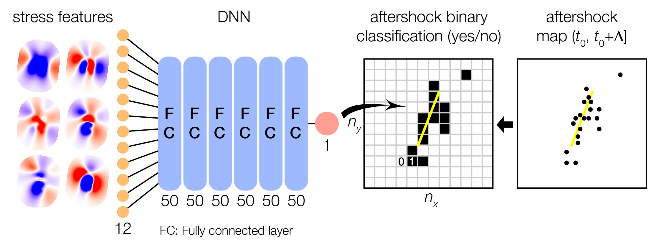
The sketch shown above illustrates their working framework. What makes this study NOT a computer vision problem is that the authors did not flatten aftershock maps as done in the computer vision applications of dense networks (see MNIST example). Instead, they defined each geographic cell as one sample, hence leading to 131,000 samples instead of 199. This means that this study was based on structured, tabulated data, made of 13 columns (12 features + 1 binary label). It was thus not recommendable to employ Deep Learning.

After exploring the neural network literature on earthquake forecasting, I only found one Deep Learning study that turns seismicity analysis into a true computer vision problem: Huang et al. (2018) transformed Taiwanese seismicity maps into images, which led to 65,536 features (corresponding to 256 × 256-pixel images). That study was, however, subject to strong under-sampling (see review in Mignan & Broccardo (2019c) and the corresponding corpus at https://github.com/amignan/hist_eq_pred).

 
A simpler alternative: A one-neuron approach by Mignan & Broccardo

The next figure shows the chronology of proposed neural network architectures, from the original DeVries et al. study to the Mignan & Broccardo ‘Matters Arising’ piece, via our conference paper. While I quickly saw that Deep Learning was not required to repeat the performance of the De Vries et al. model (simply by playing with Keras “Lego” layers – watch the technical section of the YouTube video), it took more time and the help of my colleague Marco Broccardo to figure out the obvious: A one-neuron model (i.e., logistic regression) was sufficient, with only one stress metric as input parameter, such as the sum of the absolute values of the stress change components

This result corroborates what we know from Statistical Seismology, i.e., that aftershock patterns are relatively simple.

 

 

Framing the problem by whether aftershocks are triggered by stress or strain

So far, I have restrained myself from commenting on another important aspect of the discussion, which is stress (force divided by an area) versus strain (deformation of the crust) to predict aftershocks in space, a topic certainly dear to Temblor’s readers. For stress, we need to know the stiffness of the crust, for strain we do not. The heterogeneous distribution of aftershocks in space is relatively well modelled by Coulomb stress transfer theory (King et al., 1994; Stein, 1999). DeVries et al. claimed, however, that several stress metrics, such as the sum of the absolute values of the stress components (a metric that is always positive) or the von Misses yield criterion (a square root, so also positive) are better predictors. In parallel, we know from Statistical Seismology that aftershocks are well described, at first order, by a distance power-law, considering that all aftershocks radiate homogeneously from the mainshock plane. Mignan & Broccardo (2019b) verified this by showing that using distance from mainshock rupture and mainshock mean slip as features instead of stress leads to similar results, if not better ones (again with a single neuron; see Eq. 1 of the ‘Matters Arising’ paper). There seems to be a contradiction between the stress transfer paradigm and those recent results.

Although the following hypothesis has yet to be fully tested, it is plausible that both the stress transfer theory (aftershocks in positive stress lobes) and the radial aftershock pattern are compatible, once stress changes are computed such that all the regional stress is relieved by the mainshock. This is illustrated in the next figure, where one sees how the stress field sign flips around the mainshock rupture when regional stress is fully relieved (see also Fig. 3 of King et al., 1994). Then, Coulomb stress is compatible with the observation of a radial pattern of aftershocks. If DeVries et al. modelled the other case (which is likely when looking at their extended data Figs. 2-3), Coulomb stress would perform worse than any model with positive stress around the mainshock rupture, what DeVries et al. obtained. Redoing the full stress transfer analysis of that study in this new perspective would certainly yield high Area Under the Curve scores (AUC ~ 0.85) for Coulomb stress, although this is only speculation at this point.

 

 

What is the future of Deep Learning in catastrophe risk modeling?

This article illustrated a case of unfortunate modelling strategy, rather than question the importance of Deep Learning in general, and clarified under what conditions Deep Learning should not be used. In short, Deep Learning applies best to unstructured data, such as images or waveforms. For tabulated data, simpler machine learning methods and basic regressions will often do.

Deep Learning applications in catastrophe risk modelling could include damage inference based on satellite imagery (a good example of unstructured data, which analysis is difficult to automate), although, once again, one must always remain cautious and reflect when results may be too good to be true, or are oversold (The New York Times, 2019). Every company is investigating the potential of an AI-centric view on risk, although it will certainly take several years before any robust application is proven.

There is no free lunch after all.

 
 
References
Båth M (1965), Lateral inhomogeneities of the upper mantle. Tectonophysics, 2, 483-514

Bergen KJ, Johnson PA, de Hoop MV, Beroza GC (2019), Machine learning for data-driven discovery in solid Earth geoscience. Science, 363, eaau0323, doi: 10.1126/science.aau0323

DeVries PMR, Viégas F, Wattenberg M, Meade BJ (2018) Deep learning of aftershock patterns following large earthquakes. Nature, 560, 632-634, doi: 10.1038/s41586-018-0438-y

Dieterich J (1994), A constitutive law for rate of earthquake production and its application to earthquake clustering. J. Geophys., 99, 2601-2618

Futurism (2018), Google’s AI can help predict where earthquake aftershocks are most likely, available at: https://futurism.com/the-byte/aftershocks-earthquake-prediction

Gerstenberger MC, Wiemer S, Jones LM, Reasenberg PA (2005), Real-time forecasts of tomorrow’s earthquakes in California. Nature, 435, 328-331, doi: 10.1038/nature03622

Gutenberg B, Richter CF (1944), Frequency of earthquakes in California. Bull. Seismol. Soc. Am., 34, 184-188

Hainzl S, Brietzke GB, Zöller G (2010), Quantitative earthquake forecasts resulting from static stress triggering. J. Geophys. Res., 115, B11311, doi: 10.1029/2010JB007473

Huang JP, Wang XA, Zhao Y, Xin C, Xiang H (2018), Large earthquake magnitude prediction in Taiwan based on Deep Learning neural network. Neural Network World, 2, 149-160, doi: 10.14311/NNW.2018.28.009

Kagan YY, Knopoff L (1980), Spatial distribution of earthquakes: the two-point correlation function. Geophys. J. R. astr. Soc., 62, 303-320

King GCP, Stein RS, Lin J (1994), Static Stress Changes and the Triggering of Earthquakes. Bull. Seismol. Soc. Am., 84, 935-953

Kong Q, Trugman DT, Ross ZE, Bianco MJ, Meade BJ, Gerstoft P (2019), Machine Learning in Seismology: Turning Data into Insights. Seismol. Res. Lett., 90, 3-14, doi: 10.1785/0220180259

LeCun Y, Bottou L, Bengio Y, Haffner P (1998), Gradient-Based Learning Applied to Document Recognition. Proc. IEEE, 86, 2278-2324, doi: 10.1109/5.726791

LeCun Y, Bengio Y, Hinton G (2015), Deep learning. Nature, 521, 436-444, doi: 10.1038/nature14539

Lin J, Stein RS (2004), Stress triggering in thrust and subduction earthquakes and stress interaction between the southern San Andreas and nearby thrust and strike-slip faults. J. Geophys. Res., 109, B02303, doi: 10.1029/2003JB002607

Meade, Brendan J. (2019), Reply to: One neuron versus deep learning in aftershock prediction, Nature, 574, E4, doi.org/10.1038/s41586-019-1583-7

Mignan A (2016), Revisiting the 1894 Omori Aftershock Dataset with the Stretched Exponential Function. Seismol. Res. Lett., 87, 685-689, doi: 10.1785/0220150230

Mignan A (2018), Utsu aftershock productivity law explained from geometric operations on the permanent static stress field of mainshocks. Nonlin. Processes Geophys., 25, 241-250, doi: 10.5194/npg-25-241-2018

Mignan A, Broccardo M (2019a), A Deeper Look into ‘Deep Learning of Aftershock Patterns Following Large Earthquakes’: Illustrating First Principles in Neural Network Physical Interpretability. In: Rojas I et al (ed), IWANN 2019, LNCS, 11506, 3-14, doi: 10.1007/978-3-030-20521-8_1

Mignan A, Broccardo M (2019b), One neuron versus deep learning in aftershock prediction. Nature, 574, E1-E3, doi: 10.1038/s41586-019-1582-8

Mignan A, Broccardo M (2019c), Neural Network Applications in Earthquake Prediction (1994-2019): Meta-Analytic Insight on their Limitations. preprint, arXiv: 1910.01178

Ogata Y (1998), Space-time point-process models for earthquake occurrences. Ann. Inst. Statist. Math., 50, 379-402

Omori F (1894), On after-shocks of earthquakes. J. Coll. Sci. Imp. Univ. Tokyo, 7, 111-200

Reasenberg PA, Jones LM (1994), Earthquake Aftershocks: Update. Science, 265, 1251-1252

Richards-Dinger K, Stein RS, Toda S (2010), Decay of aftershock density with distance does not indicate triggering by dynamic stress. Nature, 467, 583-586, doi: 10.1038/nature09402

Stein RS (1999), The role of stress transfer in earthquake occurrence. Nature, 402, 605-609

The New York Times (2018), A.I. Is Helping Scientists Predict When and Where the Next Big Earthquake Will Be, available at: https://www.nytimes.com/2018/10/26/technology/earthquake-predictions-artificial-intelligence.html

The New York Times (2019), This High-Tech Solution to Disaster Response May Be Too Good to Be True, available at: https://www.nytimes.com/2019/08/09/us/emergency-response-disaster-technology.html

The Verge (2018), Google and Harvard team up to use deep learning to predict earthquake aftershocks, available at: https://www.theverge.com/2018/8/30/17799356/ai-predict-earthquake-aftershocks-google-harvard

Toda S, Stein RS, Richards-Dinger K, Bozkurt SB (2005), Forecasting the evolution of seismicity in southern California: Animations built on earthquake stress transfer. J. Geophys. Res., 110, B05S16, doi: 10.1029/2004JB003415

USA Today, Harvard working with Google on AI to predict earthquake aftershocks, available at: https://eu.usatoday.com/story/tech/nation-now/2018/08/31/harvard-google-team-up-ai-predict-earthquake-aftershocks/1155203002/

Utsu TA (1961), Statistical study on the occurrence of aftershocks. Geophys. Mag., 30, 521-605

Utsu T (1970), Aftershocks and Earthquake Statistics (1): Some Parameters Which Characterize an Aftershock Sequence and Their Interrelations. J. Faculty Sci. Hookaido Univ. Series 7, Geophysics, 3, 129-195

Witze A (2018), Artificial intelligence nails predictions of earthquake aftershocks. Nature news, available at https://www.nature.com/articles/d41586-018-06091-z