Violent shaking triggers massive landslides in Sapporo Japan earthquake

Jason R. Patton, Ph.D., Ross Stein, Ph.D., Shinji Toda, Ph.D, Volkan Sevilgen, M.Sc.

The Nation of Japan is one of the most seismically active regions in the world and the people of Japan devote significant efforts to be resilient in the face of these hazards associated with earthquakes. These hazards include ground shaking, tsunami, landslides, and liquefaction. The historical knowledge of these hazards extends centuries into the past. Because of their efforts to learn using scientific methods, the world has learned more about earthquake processes.

Everyone can benefit from learning about their exposure to natural hazards from earthquakes. To learn more about your exposure to these hazards, visit temblor.net.

In this report, we discuss the ongoing earthquake sequence on the island of Hokkaido, Japan.

We emphasize here several key observations:

1. These earthquakes are related to the Hidaka Collision Zone, a convergent plate boundary that traverses the island of Hokkaido, Japan.
2. The M 6.6 earthquake shook the ground strongly, with intensity as high as JMA 6 and ground acceleration measurements as large as 1.5 g.
3. There were many earthquake triggered landslides, probably the result of colluvial slope failures. These slopes were probably preconditioned for failure due to precipitation from the recent Typhoon Jebi.
4. There were changes in tectonic stress within Earth’s interior surrounding the M 6.6 location. These changes in stress are analyzed using a computer model.

Below is a map that shows the epicenter for the mainshock, an earthquake with a magnitude M = 6.6. This map shows the coastline and active faults. There are over 700 aftershocks plotted here.

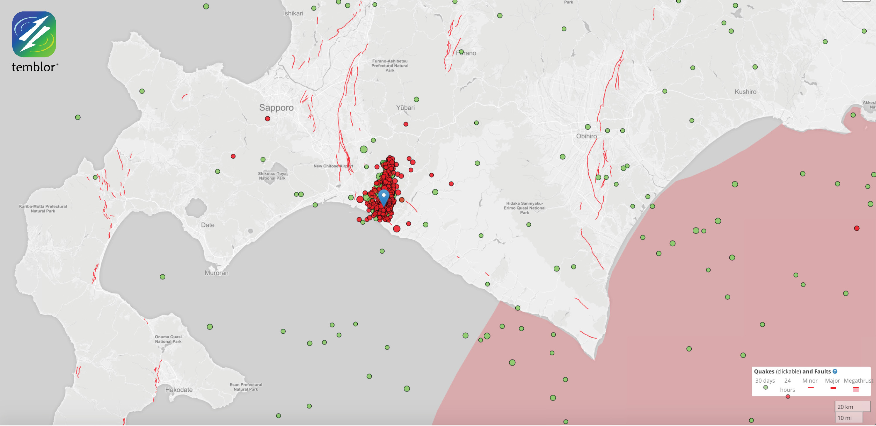
Figure 1: Regional seismicity map showing earthquake epicenters from the past 30 days. Faults are in red.

The major source of earthquakes in Japan are the numerous plate boundary fault systems, which include subduction zones, “forearc sliver” strike slip faults, and a collision zone (another form of convergent plate boundary). The figure below is from the American Geophysical Union blog “Trembling Earth,” written by Dr. Austin Elliot. Great earthquakes, quakes with M ≥ 8.0, in the 20th century include the 1923 Great Kantō subduction earthquake and the 1944 and 1946 Tōnankai and Nankai subduction earthquakes. Subduction zones are convergent plate boundaries where an oceanic plate is subducting beneath a continental or oceanic plate. These events helped shape the earth science programs in Japan, especially regarding efforts to learn about subduction zone processes. The 2011 M 9.1 Tohoku-oki subduction zone earthquake generated a trans-pacific tsunami and reminded the public that their efforts to be resilient are well founded.

 

Figure 2: Oblique view showing the configuration of the plate boundaries in the region of Japan.

The various plates and how they are configured is very complicated in Japan and we learn more about them every year. The recent M 6.6 Sapporo earthquake along the southern part of Hokkaido, Japan was also associated with a plate boundary, but not a subduction zone. In northern Japan, the North America/Okhotsk plate is moving southwestward and converging towards the Amuria/Eurasia plate. This plate motion leads to northeast-southwest oriented compression. This compression has led to the formation of tectonic deformation and thrust faults involved in the Hidaka Collision Zone. Collision zones are convergent plate boundaries where two continental plates are converging. An analogical collision zone is the collision of the India and Eurasia plates that form the Himalayas. The map below shows a generalized view of the geologic rocks in Japan, along with the location of different plate boundary faults (Van Horne et al., 2013). The Hidaka Collision Zone is labeled on the map. I placed a blue star in the location of the M 6.6 earthquake.

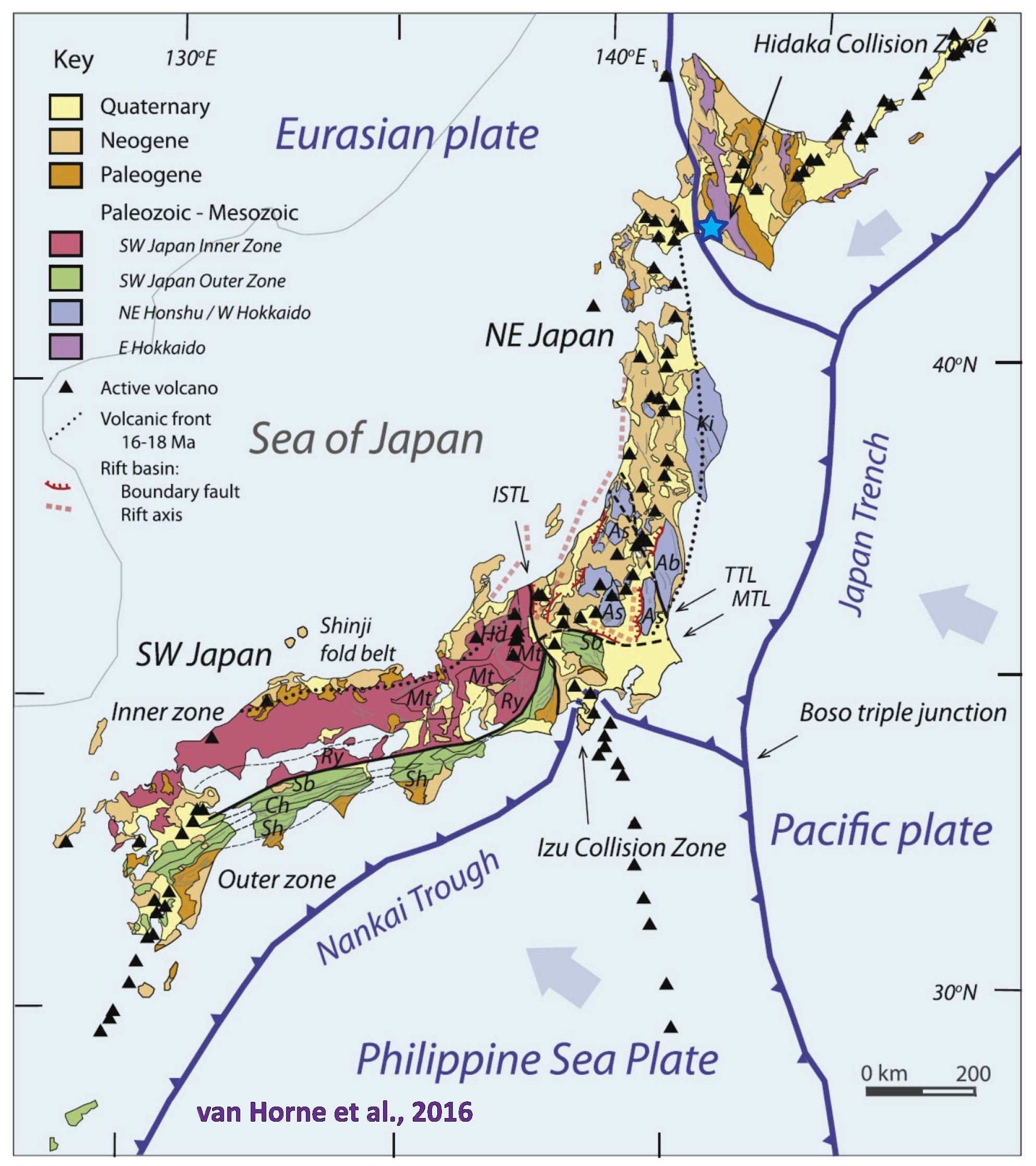
Figure 3: Geologic map of Japan showing the plate boundaries and key tectonic features including the Hidaka Collision Zone (Van Horne et al., 2016).

Ground Shaking

The M 6.6 Sapporo earthquake generated significant ground shaking and triggered landslides across the region. There are 3 main factors that control the intensity of ground shaking from earthquakes: (1) the magnitude of the earthquake, (2) the distance from the earthquake, and (3) the earth materials between the earthquake and one’s location. Earthquake magnitude is a measure of the amount of energy released during an earthquake, while intensity is a measure of how strongly the ground shakes (and how damaging the shaking is). It makes sense that when there is a larger magnitude, there is the potential for stronger shaking and a higher intensity. The magnitude does not change with distance, but intensity does. The further away from the earthquake source, the less shaking one might observe.

Here is a figure prepared using the J-SHIS Japan Seismic Hazard Information website. The color represents Peak Ground Acceleration, a measure of ground shaking. The units are also in g, an acceleration, where g = 9.8/m². If ground shaking is about 1 g, there is possibly enough energy to throw materials into the air (like rocks, cars, or buildings). The symbols represent locations where instruments made these acceleration measurements. Between symbols, the color represents an estimate of the ground shaking at those locations. Note that one site near the earthquake epicenter has a measured acceleration of 1.5 g!

Figure 4: Ground shaking map showing Peak Ground Acceleration (PGA) represented by color.

Many governments and non-governmental organizations prepare estimates of seismic hazard so that people can ensure their building codes are designed to mitigate these hazards. The Global Earthquake Model (GEM) is an example of our efforts to estimate seismic hazards, though on a global scale. Temblor.net uses the Global Earth Activity Rate (GEAR) model to prepare estimates of seismic hazard at a global to local scale (Bird et al., 2015). Each of these models incorporate earthquake information from different sources including, but not limited to, fault slip rates, records of prehistoric earthquakes, historic seismicity, and strain of the Earth’s crust as measured using Global Positioning System (GPS) observations.

Below is a map prepared using the temblor.net app. The rainbow color scale represents the chance of a given earthquake magnitude, for a given location, within the lifetime of a person. The temblor app suggests that this region could have an earthquake of M 7.1 in a human lifetime.

Figure 5: Global Earthquake Activity Rate map for this region of the northwest Pacific. Warmer colors represent regions that are more likely to experience a larger earthquake than the regions with cooler colors. Seismicity from the past is shown and the location of the M 6.6 earthquake is located near the blue teardrop symbol.

Landslides

There are many different ways in which a landslide can be triggered. The first order relations behind slope failure (landslides) is that the “resisting” forces that are preventing slope failure (e.g. the strength of the land) are overcome by the “driving” forces that are pushing this land downwards (e.g. gravity). The ratio of resisting forces to driving forces is called the Factor of Safety (FOS). We can write this ratio like this:

FOS = Resisting Force / Driving Force

When FOS > 1, the slope is stable and when FOS < 1, the slope fails and we get a landslide. The illustration below shows these relations. Note how the slope angle α can take part in this ratio (the steeper the slope, the greater impact of the mass of the slope can contribute to driving forces).

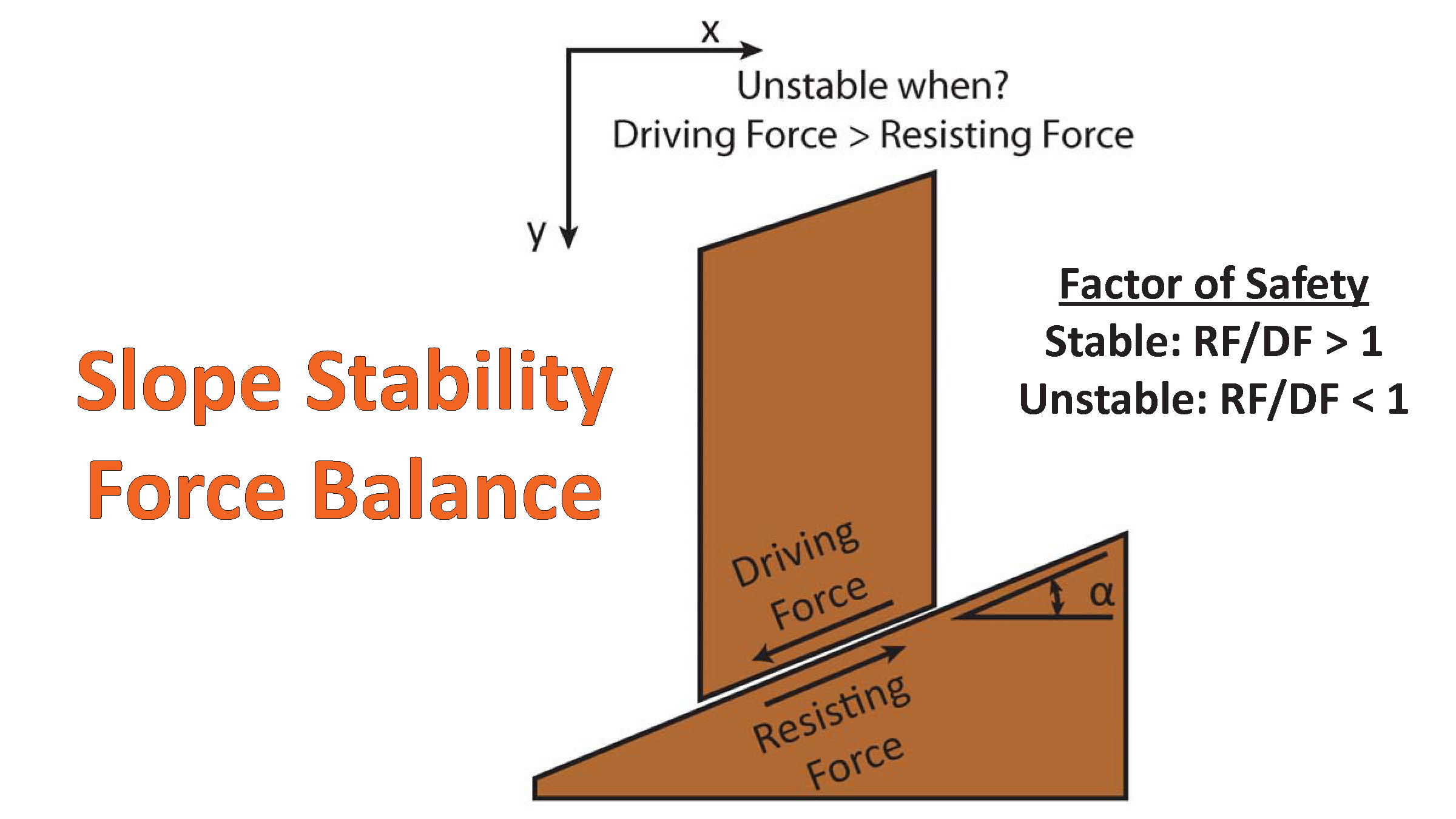
Figure 6: Landslide force balance diagram showing how driving and resisting forces balance for a stable slope.

Some factors that change this ratio include rainfall, over steepening of the slope, undercutting of the base of the slope, and earthquakes. There are other factors as well.

Japan recently experienced the most severe Typhoon in decades, which resulted in significant rainfall. When rain water infiltrates into the earth, that water can fill the spaces between soil particles and rock cracks so that the water pressure pushes apart these particles or rocks. If this pressure is large enough, the strength of the material (a resisting force) becomes weaker and there can be a landslide. Even if there is not enough reduction in resisting force, the strength of the material is still potentially weaker.

Landslide ground shaking can change the Factor of Safety in several ways that might increase the driving force or decrease the resisting force. Keefer (1984) studied a global data set of earthquake triggered landslides. The plot presented here shows that that larger earthquake magnitudes (horizontal axis) can result in landslides across a larger area.

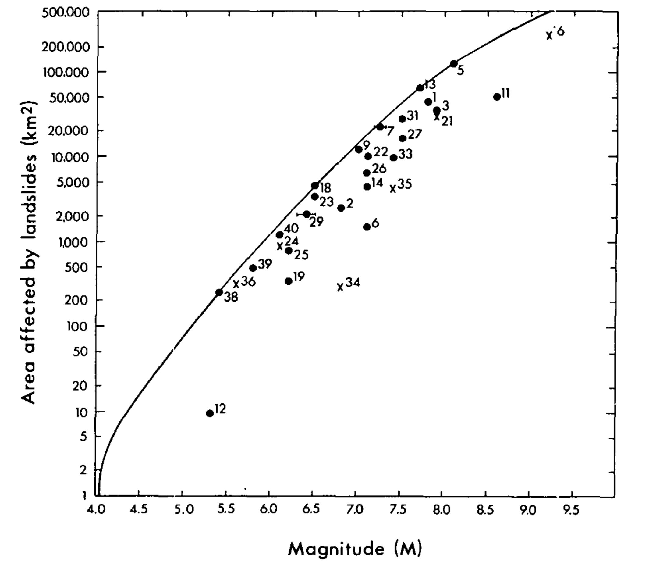
Figure 7: Spatial extent of landslide triggering by earthquakes relative to earthquake magnitude (Keefer, 1984).

As a result of the M 6.6 Sapporo earthquake, there were a large number of slope failures in the epicentral region. These landslides have covered many buildings and unfortunately have trapped many dozens of people within the debris. We will learn more about this in the coming days as search and rescue teams respond to this disaster.

There have been many videos posted online, possibly the best ones from Nippon Hōsō Kyōkai (NHK), Japan’s national public broadcasting organization. NHK also acquired the best aerial videos from the inundation of the 2011 Tohoko-oki earthquake and tsunami. There have also been some excellent comparisons between pre-landslide and post-landslide aerial imagery.

Here is a video that shows the extent of damage from some of these earthquake triggered landslides, sourced from here, from asahi.com.

Video: Aerial imagery video recorded from the Asahi Shimbun aircraft about 6 hours after the earthquake at 5 AM on 2016.09.06. This is the town of Atsuma Hokkaido.

Here is another spectacular view of some of these triggered landslides here.

Below is a pair of images that presents a comparison of the landscape from before and after the earthquake. These come from social media here.

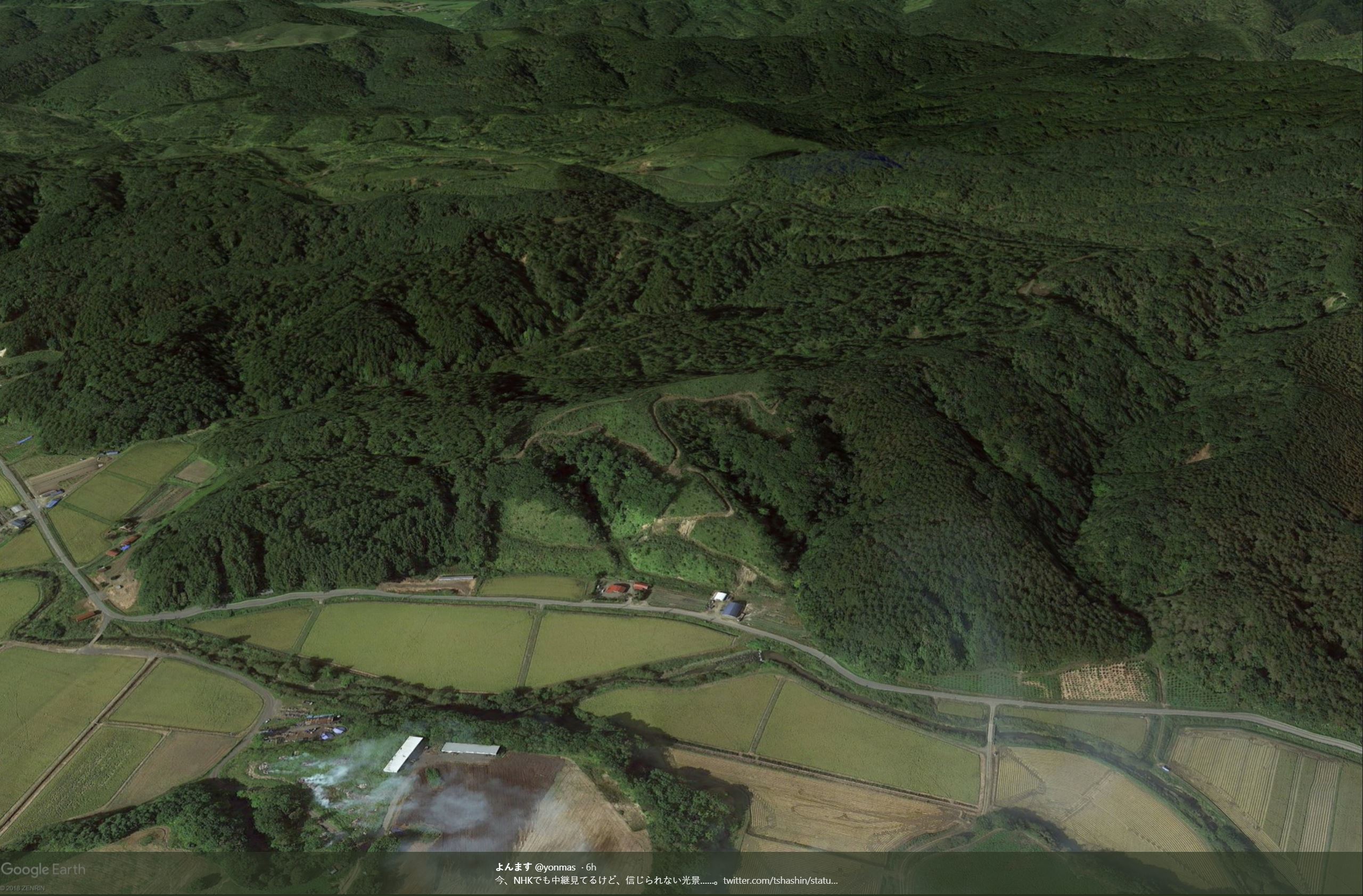
Figure 8: A comparison of imagery from before and from after the earthquake. The earthquake triggered landslides in the second image are identified in this photo by the areas of exposed brown colored soil.

These landslides appear to be failures within the soil mantle of the hillsides. While these landslides were triggered by the earthquake, it is highly likely that the water content from the Typhoon decreased the Factor of Safety prior to the earthquake. It is possible that without this preceding Typhoon, the slope failures might have been less catastrophic.

Active Faults in Hokkaido

There are a number of active crustal faults in southern Hokkaido, Japan. One may view the location of these faults on the Japan Seismic Hazard Information Station (J-SHIS) website here. In addition, estimates for seismic hazard are also placed on that website. For example, the National Seismic Hazard Map for Japan is included there. There are various versions of this map, but the most useful version is the map that shows the chance that an area in Japan will experience earthquake ground shaking at least JMA 6, for the next 30 years. The Japan Meteorological Agency Seismic Intensity Scale (JMA) is an intensity scale with a range of 0 – 7, with 7 being the highest intensity, the strongest ground shaking. To give us an idea about how strong the shaking might be for an earthquake with a JMA 6 intensity, this is what a person might experience: “Impossible to keep standing and to move without crawling.”

Below is a map that is based upon the J-SHIS website. We plot USGS earthquake epicenters from this earthquake sequence as circles colored relative to their depth with circle size relative to earthquake magnitude. Included in this map are also the active fault sources, shown as red rectangles and black lines. The two active faults in the region are different parts of the Ishikari-teichi-toen fault (the main part and the southern part). Based upon expert knowledge, these faults have the potential to produce an M 7.2 and M 7.1 earthquake for the main part and southern part, respectively. Combined, these faults may produce an M 7.9 earthquake. The USGS fault plane solution (moment tensor) is shown, along with a legend that helps one interpret this diagram. More can be found about these “beach balls” here.

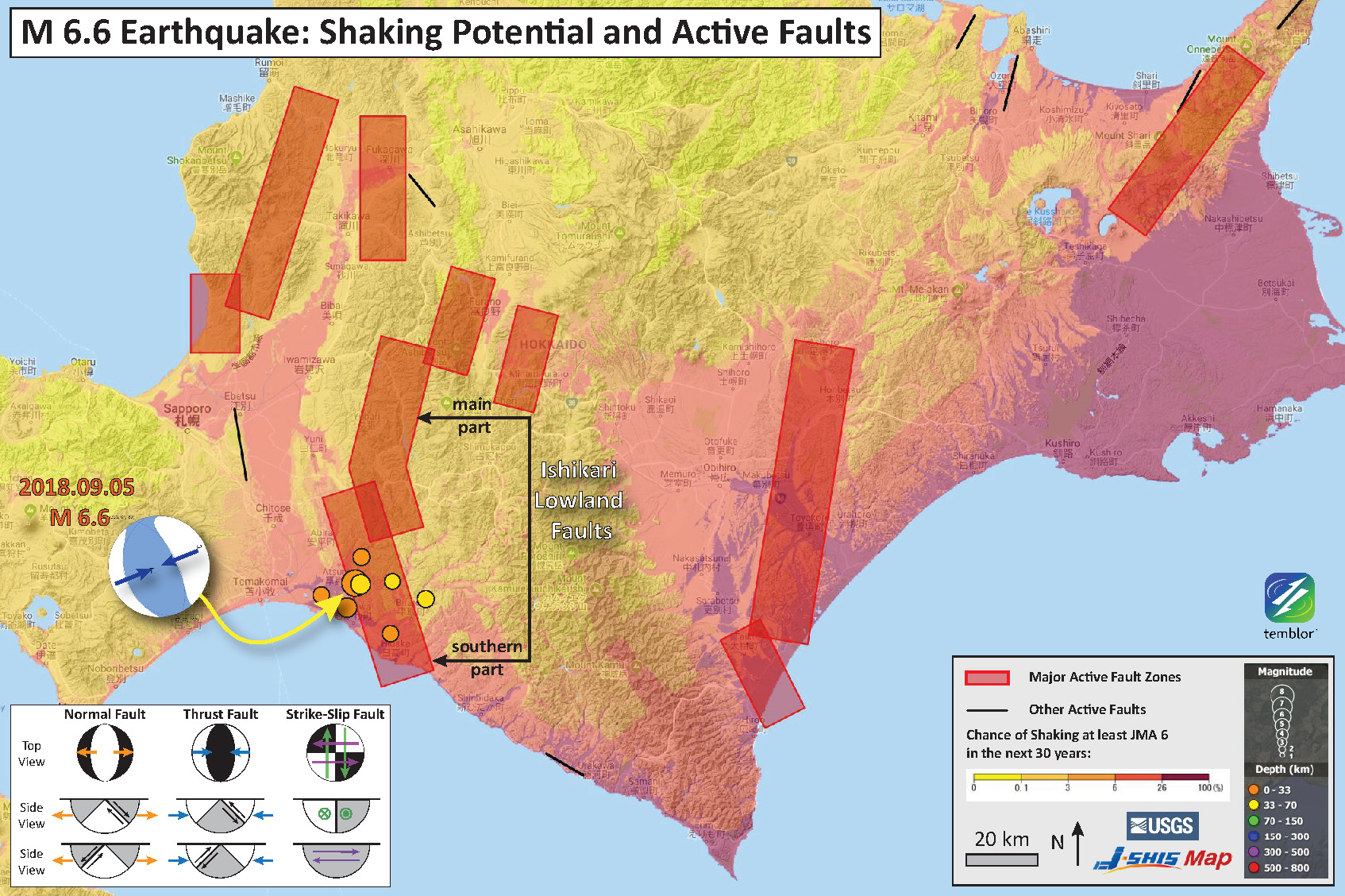
Figure 9: Earthquake shaking potential and active fault map. Warmer colors (red) represent areas that are more likely to shake strongly (minimum JMA 6) compared to the less warm colors (yellow). Active faults are shown as red rectangles or black lines.

This M 6.6 earthquake was about 33 km (20 miles) deep, deeper than the active crustal faults in the National Seismic Hazard Map. The earthquake was a thrust or reverse earthquake (oriented as a result of northeast-southwest compression, consistent with the orientation of the Hidaka Collision Zone).

This M 6.6 earthquake has changed the stresses within the crust surrounding the earthquake. The amount of this stress change is moderate, especially when compared with the amount of stress that is typically released during an earthquake. We label the faults in the above map that may or may not have an increased amount of stress (the Ishikari fault system).

This change in stress is called a change in “static coulomb stress” and a paper that discusses the fundamental factors controlling these stress increases is from Lin and Stein (2004). There is software available to the public from the USGS to perform these calculations. This software is called “Coulomb 3” and is available online here. An introduction to this software and the physics behind the calculations can be found in Stein (2003).

An earthquake occurs when the stress is greater than the strength of the rock. Rocks can have strengths that range dozens of Mega Pascal (1,000,000 Pa = 1 MPa). When earthquakes slip they release stress on the order of several to a dozen MPa. In order for an earthquake to trigger another earthquake due to these changes in stress, the triggered earthquake fault needs to have a pre-existing level of stress that is somewhat close to failure.

Dr. Shinji Toda has calculated the change in static coulomb stress as a result of the M 6.6 earthquake. They prepared two different analyses. (1) Dr. Toda first used a computer model to estimate the increased stress that could be observed on a generic fault parallel to the M 6.6 earthquake. (2) Then Dr. Toda used a computer model to estimate what the increase in stress that might be observed on a known active fault near the M 6.6 earthquake epicenter.

For both analyses, the process begins by choosing a fault geometry for the source earthquake fault (e.g. the M 6.6 earthquake fault). This includes the size (length and width) and the geometry (angle dip beneath horizontal and compass orientation) of the fault. The analysis also requires information about how much the fault slipped along this fault, which controls the magnitude of these stress changes. Finally assumptions need to be made about the material properties of the crust (i.e. the rheology), which controls the spatial distribution and extent of these stress changes. Dr. Toda used the mainshock focal mechanism and seismic moment, centered in the hypocenter

One may then calculate the change in stress on generic receiver faults in the region surrounding the source fault. Receiver faults are the faults that may have triggered earthquakes from an increase in stress. Dr. Toda calculated the change in stress for two potential source fault orientations. The figure below shows that there are regions of increased stress (red) and decreased stress (blue). The units for these stress changes are bar, a measure of force. 1 bar = 100,000 Pascal (Pa), or 0.1 MPa. If there were a fault in the red region, and this fault were parallel to the source fault, those faults have the potential to be triggered by this change in stress. Faults that are parallel to the source fault and are located in blue areas, they would have a decrease in stress, inhibiting the possibility of a triggered earthquake. Dr. Toda evaluates the results from slip on both possible nodal planes. There are two possible earthquake faults shown in fault mechanisms (the beach balls) and these two possible fault planes are called “nodal planes.”

Figure 10: Static coulomb stress change imparted by the M 6.6 earthquake onto generic receiver faults that are parallel to the source fault. Red represents regions of increased stress and blue represents regions of decreased stress.

The next step is to input the fault geometry for a “receiver” fault based upon known active faults in the National Seismic Hazard Map database. Dr. Toda selected a fault similar to the southern part of the Ishikari fault in the active fault database from Japan. The map below shows the configuration of this experiment (north is up, units on both axes is kilometers), including the shoreline and fault geometry. The source fault is the blue rectangle in the center of the map. The receiver fault is the series of small rectangles that compose a larger rectangle. Notice how the receiver fault overlaps the source fault.

Figure 11: Static coulomb stress change imparted by the M 6.6 earthquake onto an active fault with a known geometry. Red represents regions of increased stress and blue represents regions of decreased stress.

The figure here shows that there is a strong decrease in stress (-0.5 bar) in the area of the fault near the epicenter and a modest increase in stress (0.15 bar) further to the north. Drs. Toda and Stein hypothesize that the net effect probably inhibits failure on this receiver fault. The Ishikari fault is capable of producing an earthquake M > 7 and this fault did not rupture during the M 6.6 earthquake. So, those who live in the region would benefit from continuing their efforts to mitigate the earthquake hazards that they are faced with.

Here is another perspective of these data. The view is from the southeast looking into the Earth.

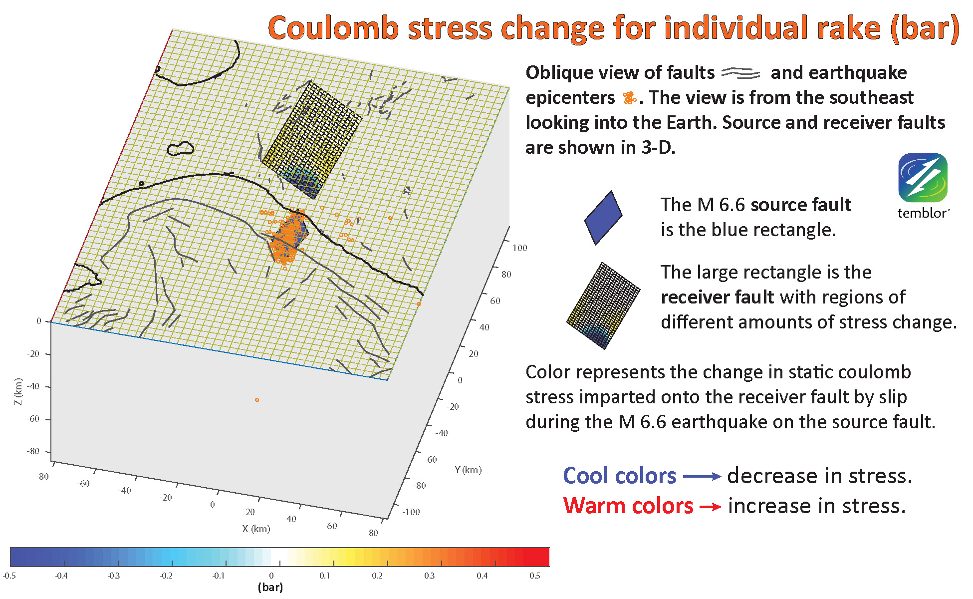
Figure 12: Low Angle Oblique Stress Changes: Static coulomb stress change imparted by the M 6.6 earthquake onto an active fault with a known geometry. Red represents regions of increased stress and blue represents regions of decreased stress.

References:

Bird, P., Jackson, D. D., Kagan, Y. Y., Kreemer, C., and Stein, R. S., 2015. GEAR1: A global earthquake activity rate model constructed from geodetic strain rates and smoothed seismicity, Bull. Seismol. Soc. Am., v. 105, no. 5, p. 2538–2554, DOI: 10.1785/0120150058

Keefer, D.K., 1984. Landslides caused by earthquakes. GSA Bulletin 95, 406-421

Lin, J., and R. S. Stein (2004), Stress triggering in thrust and subduction earthquakes and stress interaction between the southern San Andreas and nearby thrust and strike-slip faults, J. Geophys. Res., 109, B02303, doi:10.1029/2003JB002607

Stein, R.S., 2003. Earthquake conversations, Scientific American, v. 288, no. 1, p. 72-79

Travasarou, T., Bray, J.D., Abrahamson, N.A., 2003. Empirical attenuation relationship for Arias Intensity. Earthquake Engineering and Structural Dynamics 32, 1133-1155

Van Horne, A., Sato, H., Ishiyama, T., 2017. Evolution of the Sea of Japan back-arc and some unsolved issues in Tectonophysics, v. 710-711, p. 6-20, http://dx.doi.org/10.1016/j.tecto.2016.08.020

More information about the tectonics in this region can be found here.