By Zoë Mildon, Ph.D., University of Plymouth, U.K.
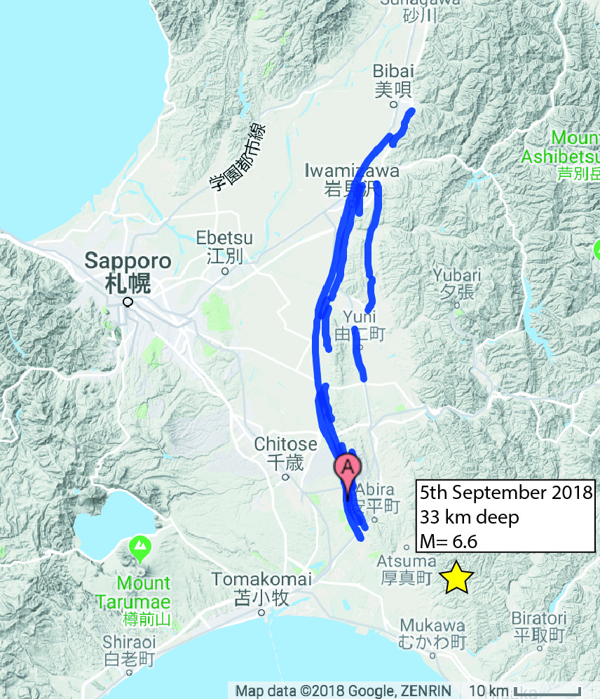
Last week, the M=6.6 Hokkaido earthquake struck the southern region of Hokkaido island, near the city of Sapporo in Japan. The earthquake caused widespread electricity blackouts and multiple large landslides.
Since then, there have been many aftershocks up to M=5.5 that have struck the region. This is fairly typical after a large earthquake, with the largest aftershock typically one magnitude unit less than the mainshock.
Where are aftershocks and subsequent mainshocks most likely to occur?
An earthquake is generated by slip on a fault (or a plane of weakness) within the crust, which causes the crust around the fault to deform, and changing the stresses in the surrounding rocks.
It is thought that by understanding these changes in stress, so-called “static stress transfer”, we may be able to understand where aftershocks are more or less likely to occur – we would expect more earthquakes to occur where the static stress has increased.
We can calculate changes in static stress using “Coulomb 3” software available from the USGS (a more detailed explanation can be found in Stein (2003)). In another Temblor blog (which you can read here), Dr. Shinji Toda presented two different models of the static stress: the first resolved onto generic parallel faults, and the second onto the known active Ishikari fault as a single planar/straight fault.
The surface trace of the Ishikari fault is slightly curved, its orientation changing along the length of the fault. This is important to know, because the amount of static stress that a fault receives depends on its orientation (e.g. Mildon et al (2016), Steacy et al (2005)). The amount of static stress is measured as a force per unit area, bars. One bar is approximately equal to atmospheric pressure at sea level.
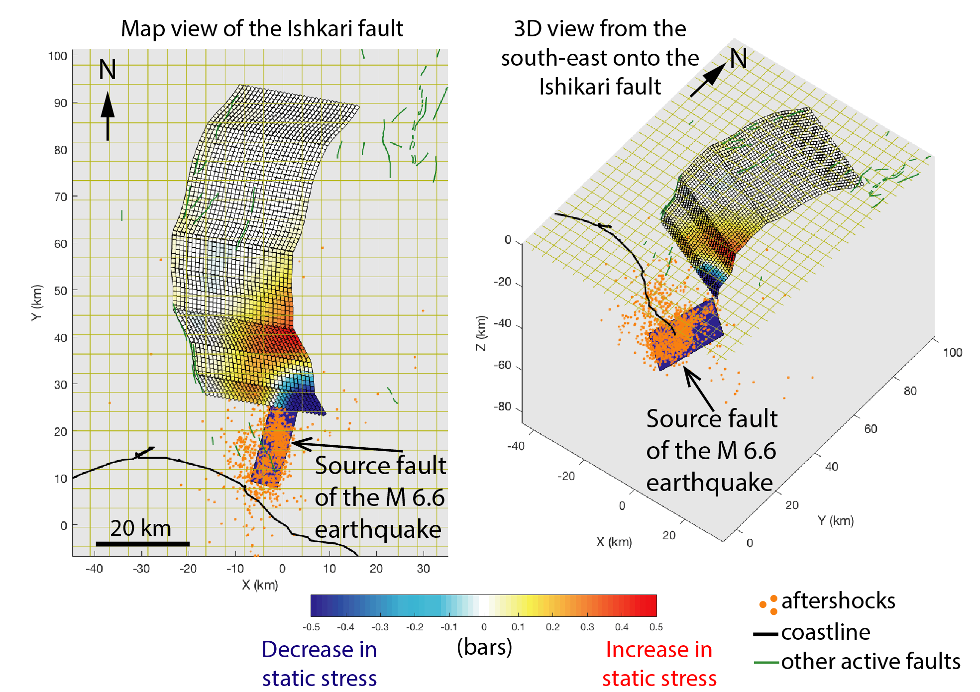
This model of the curved Ishikari fault shows that on the southern end of the fault, part of the fault that is closest to the source fault of the M 6.6 earthquake, has had a reduction in static stress (by up to -1.2 bars), which should inhibit subsequent aftershocks and mainshocks. A much larger part of the Ishikari fault is calculated to experience an increase in stress (by about +0.2 bars) – this is slightly more than calculated using a straight fault (0.15 bar).
How do the forecast compare with the first week of aftershocks?
So far, it appears that no aftershocks have stuck on the corner of the Ishikari fault calculated to have been inhibited, and several shocks have occurred on or near the part of the fault where we calculate a stress increase. So, these initial observations are consistent with the stress model.
The average or net static stress transferred across the whole Ishikari fault is -0.02 bars, which probably means that this fault is unlikely to have the timing of its next major earthquake affected by the M=6.6 shock. But considering this fault is capable of producing an earthquake M>7 event, people who live in the region should still be prepared for future earthquakes to occur.
References
Mildon, Z. K., Toda, S., Faure Walker, J. P., & Roberts, G. P. (2016). Evaluating models of Coulomb stress transfer: Is variable fault geometry important?. Geophysical Research Letters, 43(24).
Steacy, S., Nalbant, S. S., McCloskey, J., Nostro, C., Scotti, O., & Baumont, D. (2005). Onto what planes should Coulomb stress perturbations be resolved?. Journal of geophysical research: Solid Earth, 110(B5).
Stein, R.S. (2003). Earthquake conversations, Scientific American, v. 288, no. 1, p. 72-79