Introducing Coulomb 4.0: Enhanced stress interaction and deformation software for research and teaching

Temblor

3 hours ago

Figure 1. In 2023 in southeastern Turkey, two quakes struck 9 hours and 100 kilometers apart — a magnitude 7.8 event followed by a magnitude 7.7 event. Active faults, 2023 surface ruptures, background shocks and aftershocks are shown together with Coulomb stress change. One sees that seismicity has largely shut down in the (blue) stress shadows, as there are more background shocks (pink) in those regions than aftershocks (black). Many, but not all, of the (red) stress trigger zones are filled by aftershocks (black). Credit: Temblor, CC BY-NC-ND 4.0

Coulomb 4.0 is open source MATLAB software designed for interactive exploration and visualization of earthquake and volcanic processes. The software can easily incorporate ancillary data, it integrates the ISC earthquake toolbox and USGS finite fault models, and produces publication-ready graphics.

By Kaede Yoshizawa, Tohoku University, Japan, Shinji Toda Tohoku University, Japan,
Ross S. Stein, Temblor, Inc., USA, Volkan Sevilgen, Temblor, Inc., USA, and Jian Lin, Southern University of Science and Technology, PRC

Citation: Yoshizawa, K., Toda, S., Stein, R. S., Sevilgen, V., Lin, J., 2026, Introducing Coulomb 4.0: Enhanced stress interaction and deformation software for research and teaching, Temblor, http://doi.org/10.32858/temblor.372

Faults converse with one another by the transfer of stress. This can occur in several ways. Static elastic stress changes are permanent. Viscoelastic stress is transmitted by flow in the lower crust. Poroelastic stress occurs through diffusion of fluids in the upper crust. Dynamic stress is carried by seismic waves excited by a mainshock; the imparted stresses are large but transient, disappearing in minutes to hours.

Coulomb 4.0, an updated version of Coulomb 3.4, enables exploration of the first — and we believe, the most important — of these interactions. One can quickly make idealized but realistic calculations, such as tapered slip on a rectangular patch with size appropriate for an earthquake magnitude. But more complex and detailed calculations are also possible, such as using USGS finite fault models, which break the fault plane into patches, each with its own amount of slip and rake (direction of slip).

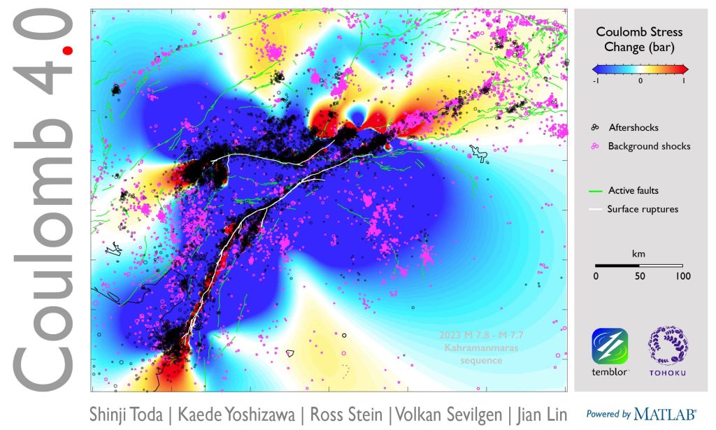
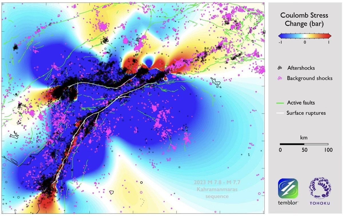
Coulomb 4.0 places the greatest emphasis on a user building their intuition and understanding by starting simply and progressing to more realism, all the while examining the results in 2D and 3D, in map view and cross-section (Figure 1). Compared to its predecessor, Coulomb 4.0 unifies all calculations, earthquake catalog, map overlays, and visualizations into a single seamless workspace. So, all calculation options are visible, with nothing hidden behind pop-up menus.

An ideal teaching tool

Simple tools make Coulomb 4.0 an ideal teaching platform to explore crustal deformation and stress transfer. The ability to build simple rectangular faults or dikes with tapered slip, and then examine the shear and normal stress they impart to their surroundings, in map view or cross-section, enable the user to develop valuable intuition and insights about stress transfer.

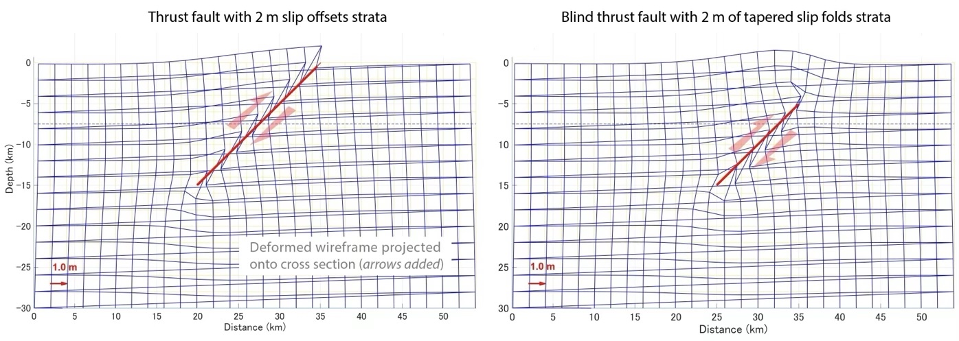
One can also use Coulomb 4.0 to explore concepts and features of crustal deformation. For instance, in Figure 2, we can see the impact on the upper crust of a thrust fault that cuts the surface (left panel) or is buried (right panel). A 45°-dipping fault has the greatest deformation asymmetry of deformation. A 45°-dipping thrust, as shown in Figure 2, produces the greatest net uplift; a 45°-dipping normal fault produces the greatest net subsidence.

Figure 2. A deformed wireframe illustrates surface folding associated with a thrust fault. On the left, the fault ruptures the surface. On the right, the fault does not reach the surface. The deformation shown in both panels has been exaggerated by a factor of 1,000 to show 2 kilometers of cumulative slip in an elastic medium. Poisson’s ratio has been changed from the 0.25 default to 0.5 so that volume is preserved. This makes cross-sections ‘retrodeformable,’ meaning the deformation can be undone and the strata restored, as generally assumed by geologists for the lithosphere. Credit: Temblor, CC BY-NC-ND 4.0

An intuitive workspace

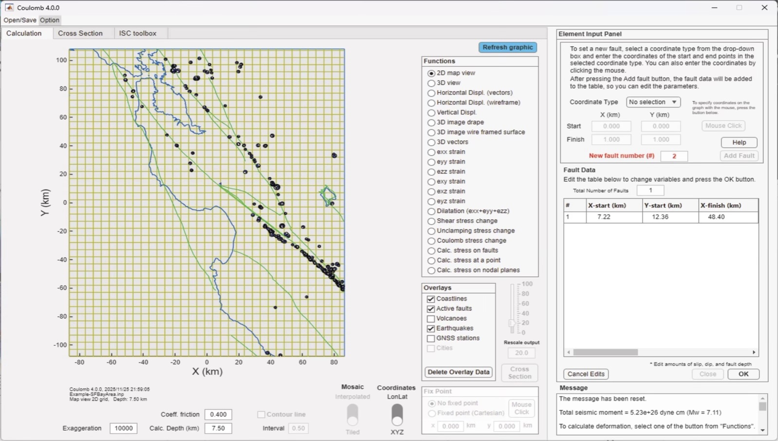
Coulomb 4.0 now uses a single workspace (Figure 3) that makes all options evident to the user. One can build source or receiver faults directly on the map, adding slip and rake — eliminating switching between screens, and so speeding and simplifying the analysis.

Figure 3. Coulomb 4.0’s updated desktop, with a map, Functions, Overlays and the Element Input Panel all simultaneously visible. One can toggle between Mosaic and Interpolated stress or strain. Contours can be added. The fault friction coefficient, calculation depth exaggeration can be adjusted. Whenever one inputs an earthquake source and slip, its seismic moment and magnitude (Mw) is reported in the Message panel. Credit: Temblor, CC BY-NC-ND 4.0

Incorporating the ISC Earthquake Toolbox

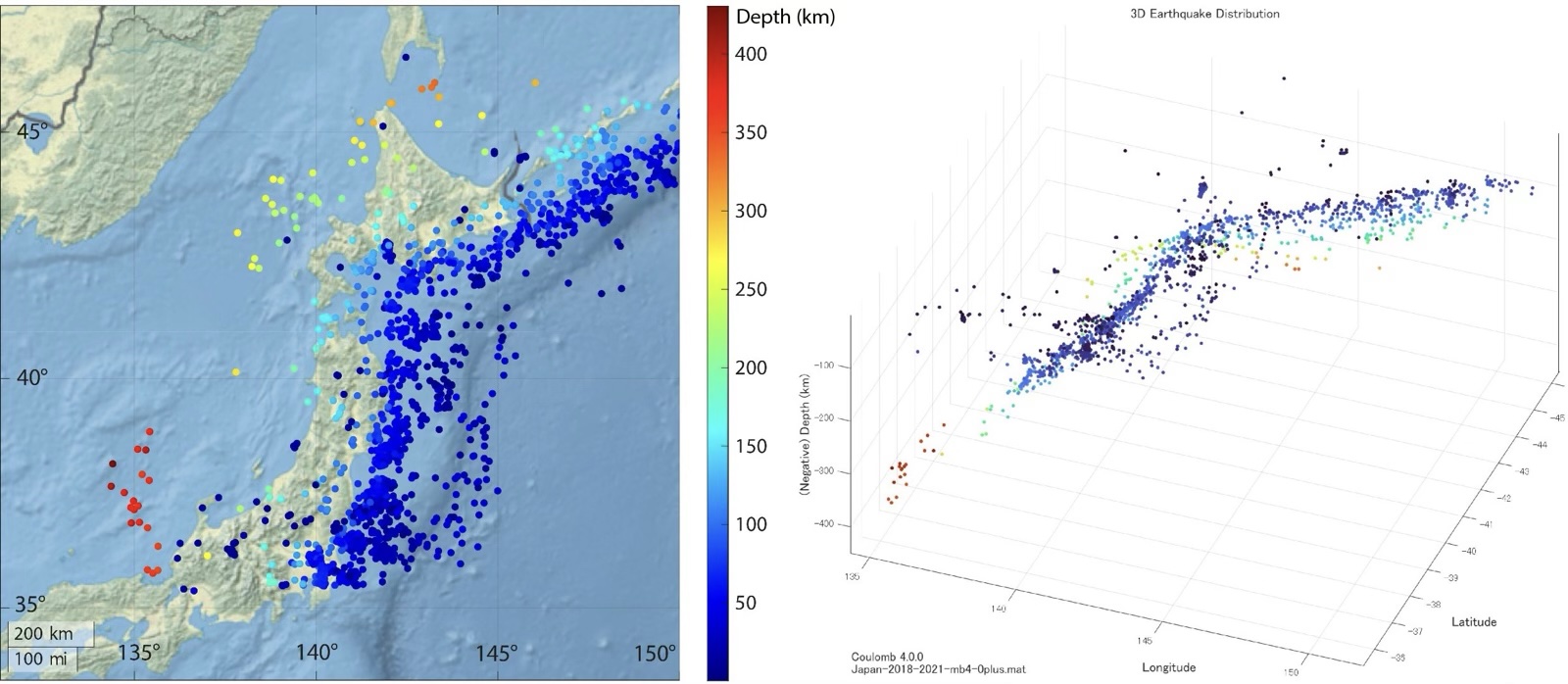
We have designed Coulomb 4.0 to allow the ISC (International Seismological Centre) earthquake catalog to operate within the software (Figure 4). This and other global catalogs now sit in the same workspace as stress change modeling. In particular, ISC earthquakes can be filtered by time, magnitude, depth, and region, then instantly plotted on stress change maps and in 3D to test whether seismicity corresponds to modeled stress changes.

Figure 4. Coulomb 4.0 incorporates the ISC catalog for easy comparison of earthquakes with stress changes. On the left panel, seismicity in Japan is colored by depth. On the right panel, we see the same earthquakes in a 3D view that can be spun or zoomed while on the screen. Credit: Temblor, CC BY-NC-ND 4.0

Building fault sources and receivers

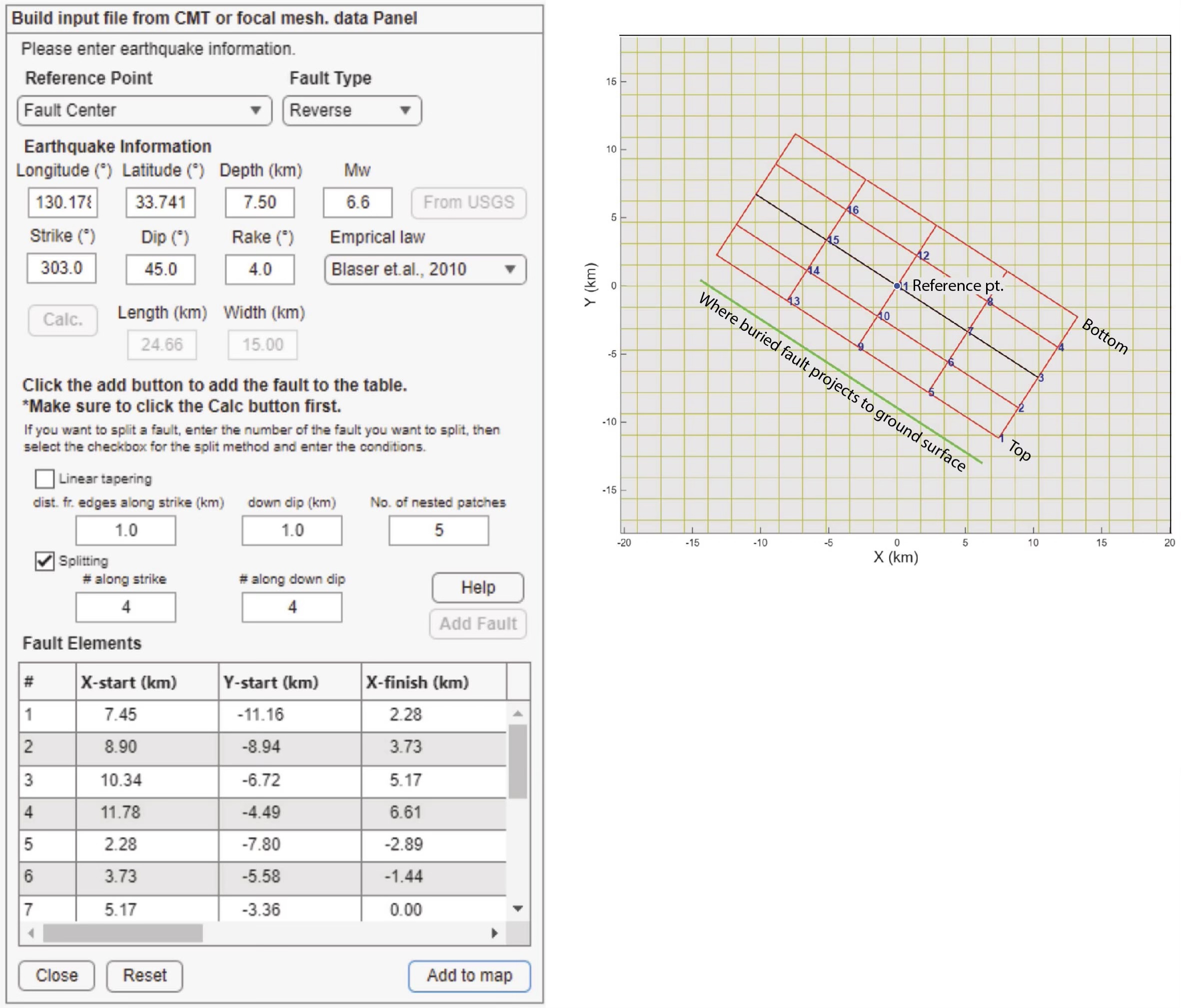
Fault sources and receivers can be built directly from centroid moment tensors (CMTs) or with map clicks. Coulomb 4.0 includes Blaser et al. (2010) or Wells & Coppersmith (1994) empirical scaling of magnitude to source dimensions and slip.

Tapering is valuable for source faults, providing more realistic stress transfer to nearby receiver faults. Tiling the fault surface is valuable when exploring receiver faults, so one can see how the stress varies over the fault surface. Coulomb 4.0 allows both (Figure 5)

Figure 5. The ‘Build input file from CMT or focal mechanism’ data panel makes it easy to add sources or receivers. The amount of tapering and the number of tiles can be adjusted by the user. Credit: Temblor, CC BY-NC-ND 4.0

Viewing results in different ways

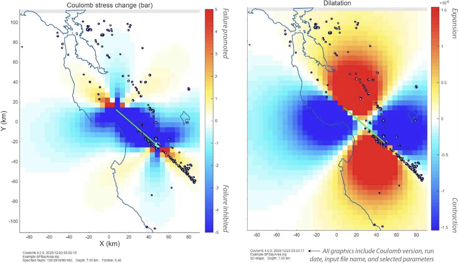
The clean, intuitive interface enables users to view and manipulate results. In particular, users can move between map (Figure 6), 3-D deformation, displacement vectors (Figure 7), wireframes, strain, and stress change views with ease. For example, in Figure 6, we show the stress imparted by a simplified source for he 1989 magnitude 6.9 Loma Prieta, California, earthquake. The left panel shows Coulomb stress, with may most affect fault creep and seismicity. The right panel shows dilatation, which may influence fluid diffusion.

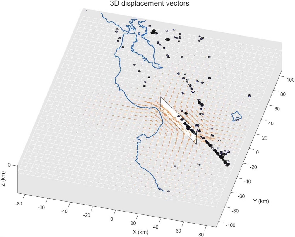
Figure 6. Coulomb stress (left) and dilatation (right) caused by the same simplified source, the 1989 magnitude 6.9 Loma Prieta earthquake. These comparisons can help assess which is better correlated with subsequent seismicity or fault creep. Credit: Temblor, CC BY-NC-ND 4.0

But note how, for the same example, plotting surface displacements on a regular grid reveals an arc-like pattern of vectors. In Coulomb 4.0, one could easily import the observed GPS displacements and compare them to the modeled vectors, enabling the user to develop intuition about displacement.

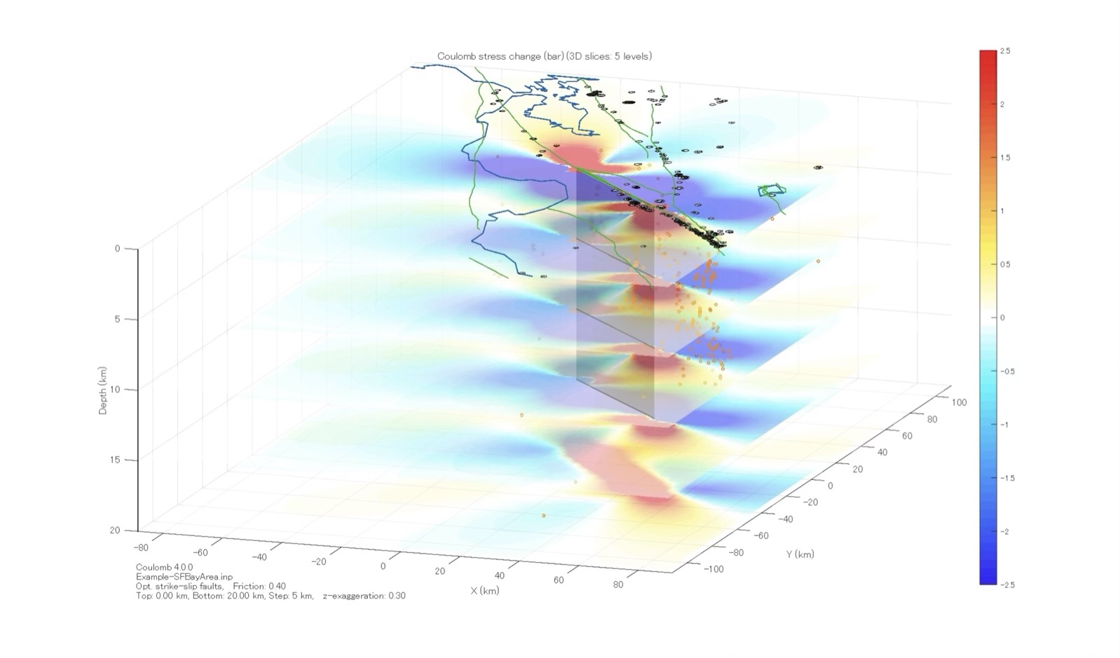
Figure 7. Surface displacements for the vertical right-lateral rupture shown in Figure 6 reveal the arc-like pattern of vectors, which are only aligned parallel to the fault near its center. Credit: Temblor, CC BY-NC-ND 4.0

Stress change with depth

Through cross sections, Coulomb 4.0 can reveal stress change as a function of depth. In addition, a new depth-loop engine produces stress change at multiple depths. These new functions enable iso-surfaces, vertical slices, and horizontal slices (Figure 8) which can be helpful for understanding the 3D distribution of stress changes.

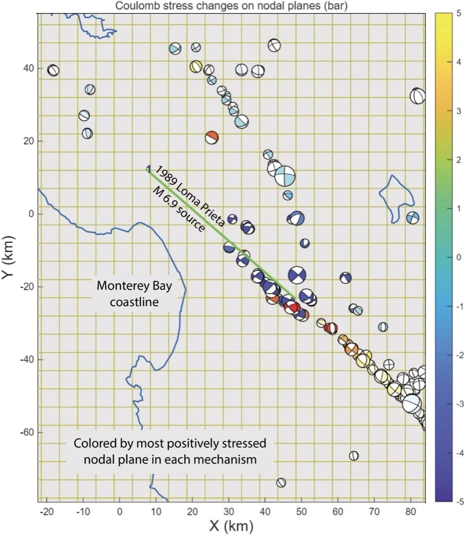
Figure 8. This image shows how stress changes with depth down to 20 kilometers. Earthquakes are plotted in black on the top surface, and earthquake depth bands are repeated in orange at each depth slice. Credit: Temblor, CC BY-NC-ND 4.0

Imparting stress to nodal planes

Faults, coastlines, and volcanoes can be easily overlain. To compare modeled stresses with observed rupture styles, earthquake catalogs can be filtered and sorted, with ‘beachballs’ color-coded by stress change (Figure 9). Coulomb stress will only be the same on both nodal planes if friction were zero. So, one can select and plot the most positively-stressed nodal plane, or Coulomb 4.0 can randomly select the nodal planes.

Figure 9. Coulomb stress imparted to surrounding earthquakes using a simplified 1989 Loma Prieta earthquake source. Red mechanisms are promoted toward failure; blue mechanisms are inhibited. So, one would expect seismicity after the 1989 quake to turn off where beachballs are blue, and turn on where they are red. Credit: Temblor, CC BY-NC-ND 4.0

Animated swiveling GIFs are easy to make

Sometimes seeing the stress or seismicity from several angles reveals relationships hidden in 2D plots. To that end, Coulomb 4.0 allows users to make moving 3D images (Figure 10).

Figure 10. This GIF, which is easily created in Coulomb 4.0, shows the distribution of Coulomb stress imparted by the 2025 magnitude 8.8 Kamchatka rupture (the surface-cutting megathrust fault) to the fault plane of the largest aftershock (the smaller, deeper rectangle with a finer mesh), where the stress was generally increased by a few bars. Credit: Temblor, CC BY-NC-ND 4.0

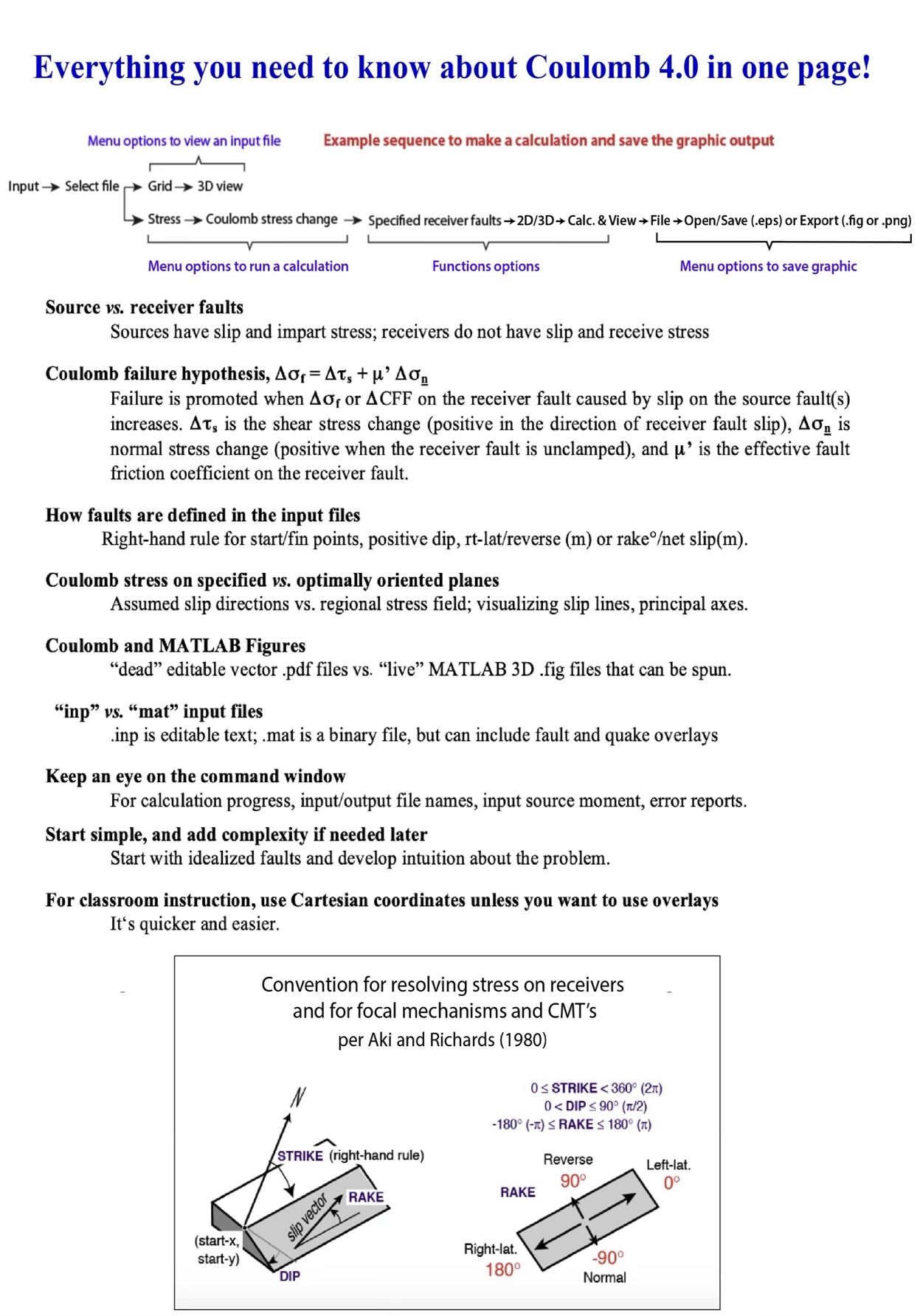
No manual!

We have tried to show explanations on the screen as actions are taken. Otherwise, we have boiled it all down to one page (Figure 11).

Figure 11. Everything you need to know about Coulomb but were afraid to ask. Credit: Temblor, CC BY-NC-ND 4.0

Conclusion

Coulomb 4 uses the MATLAB Mapping Toolbox, the Image Processing Toolbox, and the Curve Fitting Toolbox. Most universities and some companies have MATLAB licenses. We hope Coulomb 4 will find its way into college classrooms, research groups, and journal publications. Its predecessor, Coulomb 3, has been downloaded 10,000 times and cited in 3,000 journal articles. We look forward to similar adoption of Coulomb 4.

Coulomb 4.0 download

https://temblor.net/coulomb/

https://github.com/YoshKae/Coulomb_Update

Acknowledgements

We thank MathWorks for a software development grant to Temblor, and Kostas Leptokaropoulos and Lisa Kempler from MathWorks for their invaluable guidance.

References

Blaser, L., Krüger, F., Ohrnberger, M., & Scherbaum, F. (2010). Scaling relations of earthquake source parameter estimates with special focus on subduction environment. Bulletin of the Seismological Society of America, 100(6), 2914-2926.

Wells, D. L., & Coppersmith, K. J. (1994). New empirical relationships among magnitude, rupture length, rupture width, rupture area, and surface displacement. Bulletin of the seismological Society of America, 84(4), 974-1002.

Copyright

We publish our work — articles and maps made by Temblor — under a Creative Commons Attribution-NonCommercial-NoDerivatives 4.0 International (CC BY-NC-ND 4.0) license.

For more information, please see our Republishing Guidelines or reach out to news@temblor.net with any questions.